B Aim2: BOUNCEBACK RESILIENCE
rm(list=ls())

library(raster)
library(sf)
library(rasterVis)
library(tidyverse)
library(haven)
library(stringr)
library(scales)
library(colorspace)
library(MASS)
B.1 Visuals
a <- dat_year %>%
  #filter(!is.na(nl_viirs_2)) %>%
  filter(year>2011, year<2019) %>%
  ungroup() %>%
  group_by(id_loc) %>%
  mutate(nl_viirs_2.baseline = first(nl_viirs_2),
         VIIRS = cut(nl_viirs_2.baseline, breaks=c(-Inf,5,Inf)),
         MEI_ike_udel.baseline = first(MEI_ike_udel),
         MEI = cut(MEI_ike_udel.baseline, breaks=c(-Inf,0.6,Inf)),
         cat = paste0(VIIRS,MEI))
B.1.1 vivax malaria
P. vivax malaria trends relative to MEI and VIIRS categories at baseline (2012). Each line represents a location (village).
a %>%
  ggplot(aes(x = year, y = viv_rate, group=id_loc, col = factor(cat))) +
  geom_point() +
  geom_line() +
  theme_bw() +
  scale_color_discrete_sequential(palette = "Red-Blue") +
  guides(col=F) +
  labs(y="Malaria rate") +
  facet_grid(VIIRS~MEI, labeller=label_both)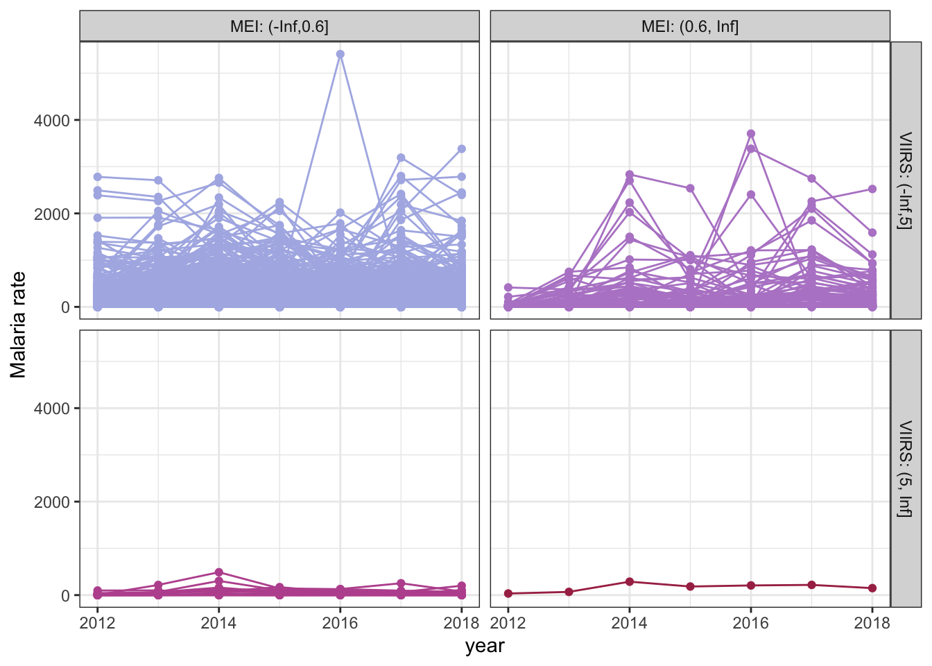
B.1.2 falciparum malaria
P. falciparum malaria trends relative to MEI and VIIRS categories at baseline (2012). Each line represents a location (village).
a %>%
  ggplot(aes(x = year, y = fal_rate, group=id_loc, col = factor(cat))) +
  geom_point() +
  geom_line() +
  theme_bw() +
  scale_color_discrete_sequential(palette = "Red-Blue") +
  guides(col=F) +
  labs(y="Malaria rate") +
  facet_grid(VIIRS~MEI, labeller=label_both)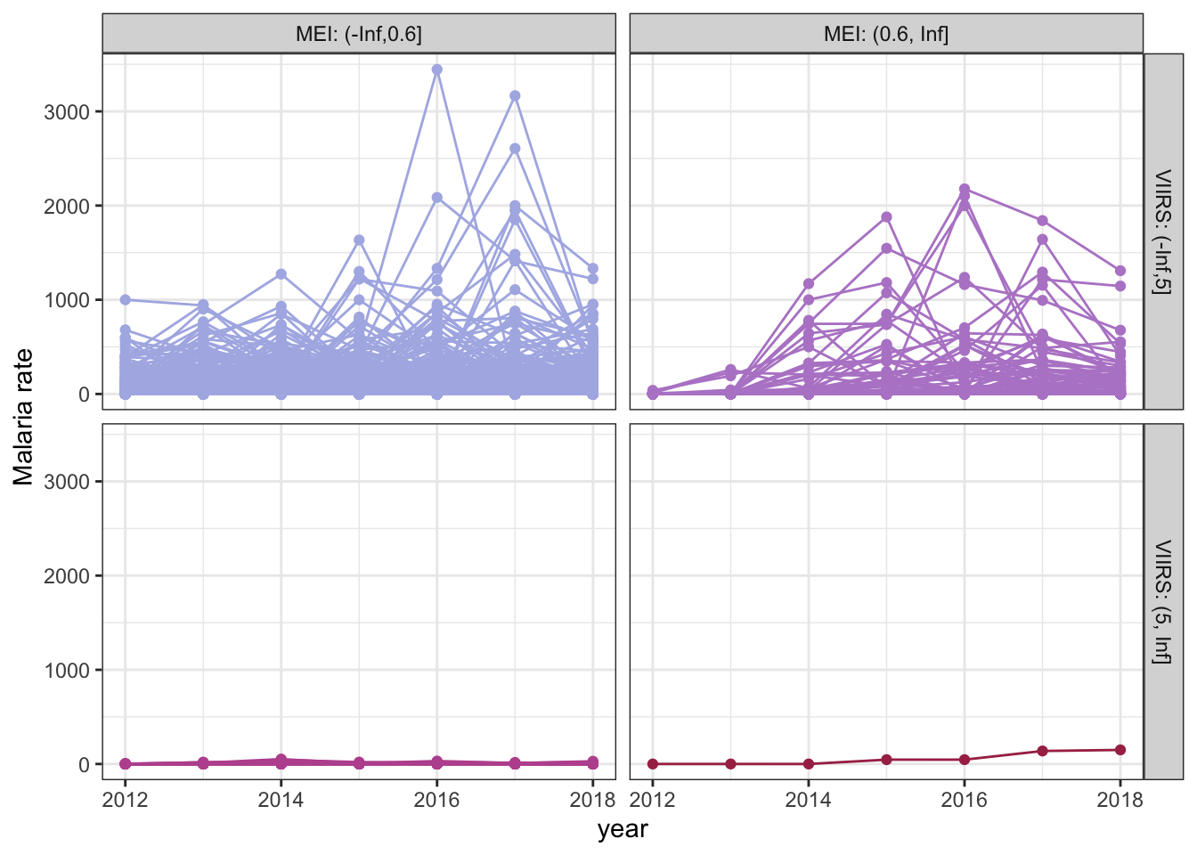
B.2 Slope calcualtions
A negative binomial model per location.
c<-glm.nb(viv ~ year, data = a, na.action=na.exclude)
c$coefficients[2] <-NA
glm.nb.safe <- possibly(glm.nb, otherwise = c)

dt_s <- dat_year %>%
  filter(year>2011, year<2019) %>%
  ungroup() %>%
  #filter(NOMBDIST=="IQUITOS") %>%
  dplyr::select(id_loc, year, viv, fal, nrohab) %>%
  gather(var, value, viv:fal) %>%
  nest(-id_loc, -var) %>%
  mutate(model = map(data, ~glm.nb.safe(value ~ year + offset(log(nrohab)), data = ., na.action=na.exclude)),
         slope = lapply(model, function(x) { x$coefficients[2] })) %>%
  dplyr::select(id_loc, var, slope) %>%
  unnest(cols = c(slope)) %>%
  spread(var,slope) %>%
  rename(slope_fal = fal, slope_viv = viv)

dt_s.c <- a %>%
  filter(year==2012) %>%
  inner_join(dt_s, by="id_loc") %>%
  inner_join(st_set_geometry(dat, NULL) %>%
  filter(year==2012) %>%
  distinct(id_loc, .keep_all = T), by="id_loc")
B.2.1 vivax malaria
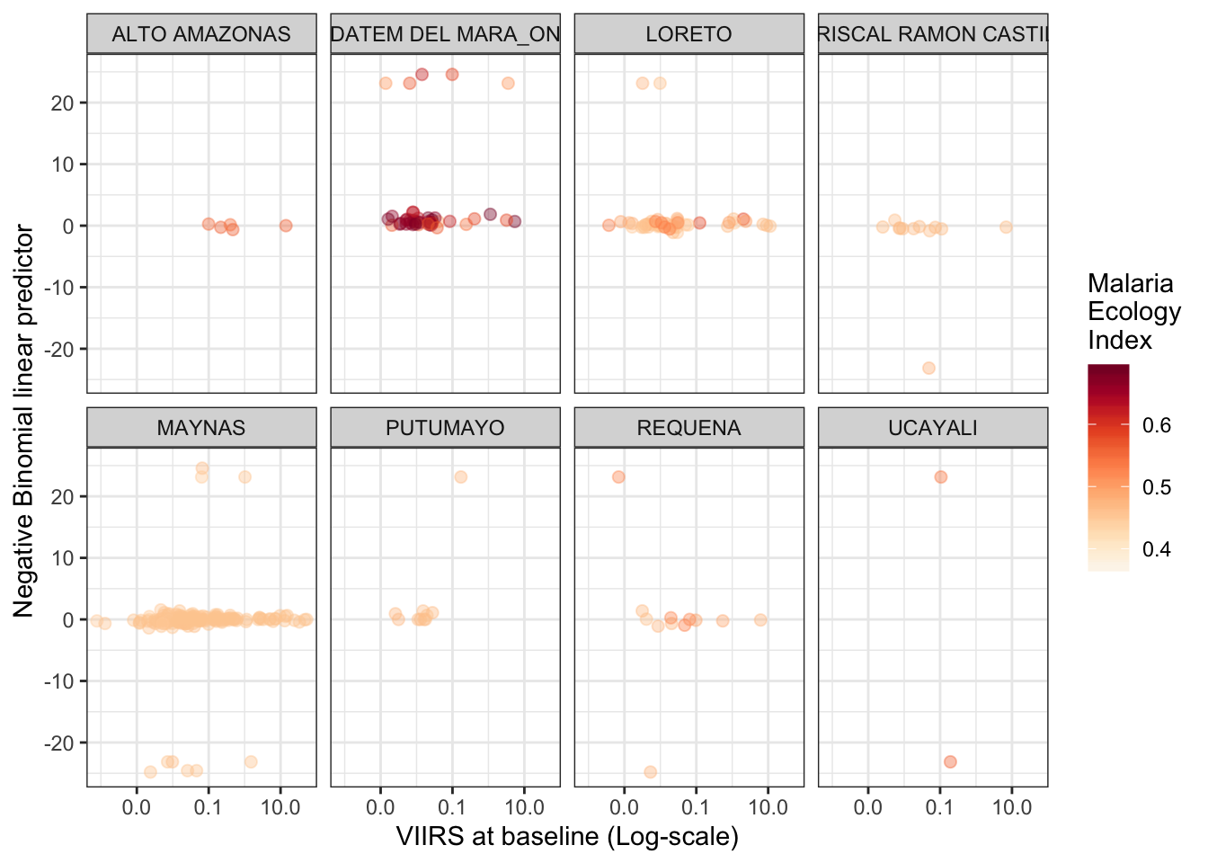
Plotting the slope (linear predictor) vs. VIIRS at baseline
dt_s.c %>%
  ggplot(aes(y = slope_viv, x = nl_viirs_2.baseline, col = MEI_ike_udel.baseline)) +
  geom_point(size = 2, alpha=.4) +
  scale_x_log10(label = number_format(accuracy = .1)) +
  labs(y= "Negative Binomial linear predictor", x = "VIIRS at baseline (Log-scale)", col = "Malaria\nEcology\nIndex") +
  scale_color_continuous_sequential(palette = "OrRd") +
  theme_bw() +
  facet_wrap(province.x~., ncol = 4)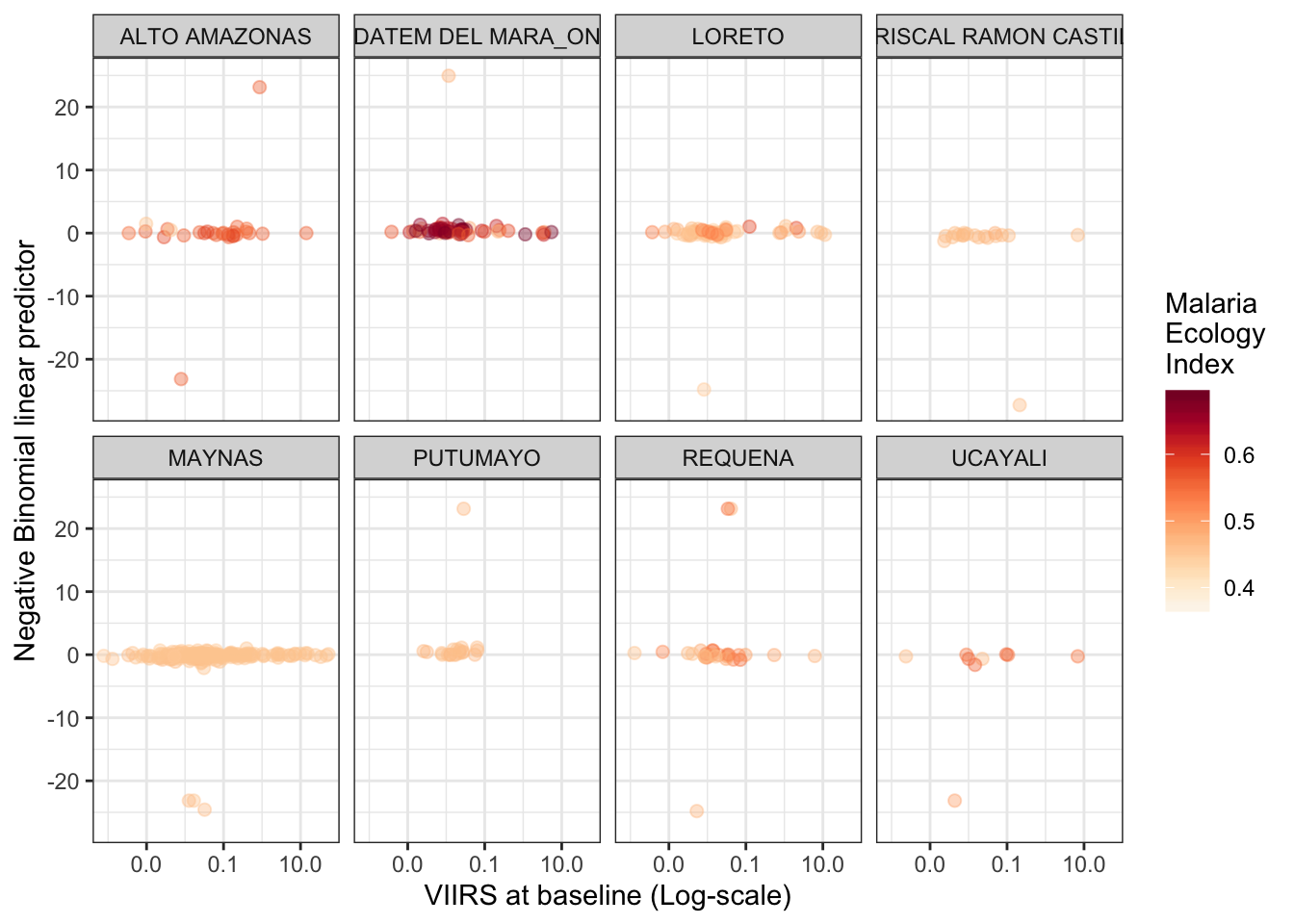
B.2.2 falciparum malaria
Plotting the slope (linear predictor) vs. VIIRS at baseline
dt_s.c %>%
  ggplot(aes(y = slope_fal, x = nl_viirs_2.baseline, col = MEI_ike_udel.baseline)) +
  geom_point(size = 2, alpha=.4) +
  scale_x_log10(label = number_format(accuracy = .1)) +
  labs(y= "Negative Binomial linear predictor", x = "VIIRS at baseline (Log-scale)", col = "Malaria\nEcology\nIndex") +
  scale_color_continuous_sequential(palette = "OrRd") +
  theme_bw() +
  facet_wrap(province.x~., ncol = 4)