Chapter 3 Aim1: PREDICTION CAPACITY

rm(list=ls())

library(raster)
library(sf)
library(rasterVis)
library(tidyverse)
library(haven)
library(stringr)
library(scales)
library(cowplot)
library(ggpubr)

dat <- readRDS(file.path(wd, "/dat_NL_MAL.RData")) %>%
  filter(nrohab>20) %>%
  mutate(fal_rate = 100*fal/nrohab,
         viv_rate = 100*viv/nrohab)

dat_year <- dat %>%
  ungroup() %>%
  group_by(year, id_loc) %>%
  filter(nrohab>20) %>%
  summarise(fal = sum(fal),
            viv = sum(viv),
            nrohab = mean(nrohab),
            MEI_ike_udel = mean(MEI_ike_udel),
            nl_viirs_2 = mean(nl_viirs_2, na.rm=T)) %>%
  mutate(fal_rate = 1000*fal/nrohab,
         viv_rate = 1000*viv/nrohab) 

3.1 Visuals

3.1.1 Montly malaria cases

dat %>%
  gather(spp, rate, fal_rate:viv_rate) %>%
  arrange(MEI_ike_udel)%>%
  filter(year>2011, year<2018) %>%
  #filter(rate<4000) %>%
  ggplot(aes(nl_viirs_2, rate, col = MEI_ike_udel)) +
  geom_point(alpha=.7) +
  #scale_y_continuous(label = math_format())
  scale_y_log10(label = number_format(accuracy = .1)) +
  scale_color_distiller(palette = "OrRd", direction=1) +
  geom_smooth(linetype = "dashed", color ="#5C5C5C") +
  theme_bw() +
  labs(x = "Nighttime Lights (radiance values)", y= "Monthly Malaria Rate (x100 hab.)", color = "Malaria\nEcology\nIndex") +
  facet_grid(.~spp, labeller = labeller(spp=c(fal_rate = "falciparum", viv_rate = "vivax")))

3.1.2 Yearly malaria cases

dat_year %>%
  gather(spp, rate, fal_rate:viv_rate) %>%
  arrange(MEI_ike_udel)%>%
  filter(year>2011, year<2018) %>%
  #filter(rate<4000) %>%
  ggplot(aes(nl_viirs_2, rate, col = MEI_ike_udel)) +
  geom_point(alpha=.7) +
  #scale_y_continuous(label = math_format())
  scale_y_log10(label = number_format(accuracy = .1)) +
  scale_color_distiller(palette = "OrRd", direction=1) +
  geom_smooth(linetype = "dashed", color ="#5C5C5C") +
  theme_bw() +
  labs(x = "Nighttime Lights (Averaged radiance values)", y= "Annual Malaria Rate (x100 hab.)", color = "Averaged\nMalaria\nEcology\nIndex") +
  facet_grid(.~spp, labeller = labeller(spp=c(fal_rate = "falciparum", viv_rate = "vivax")))

3.2 Linear Probability model

STATA specification

import delimited "/Users/gcarrasco/Dropbox/Work/Colabs UCSD/Malaria & Develop [McCord]/Data/dat_NL_MAL_stata.csv", clear

collapse (sum) viv fal (max) bin_viv bin_fal viirs=nl_viirs_2 mei_ike_udel (first) provincex, by(year id_loc)

encode id_loc, gen(id)
xtset id

summ viirs, d
drop if viirs==.
drop if viirs>11.45

gen viirs2 = viirs^2

3.2.1 Model vivax

p <- dat %>% ggplot(aes(y=bin_viv, x=nl_viirs_2)) +
  geom_hline(yintercept=c(0,1), linetype = "dashed", col = "red") +
  geom_point(alpha=.6) + 
  geom_smooth(method = "lm", col = "blue", fill="blue") +
  geom_smooth(method = "glm", method.args = list(family = "binomial"), col="red", fill="red") +
  theme_classic()

xplot <- ggdensity(dat, "nl_viirs_2") +
  labs(x="")

plot_grid(xplot, p, ncol = 1, align = "hv", rel_heights = c(1, 2))

In STATA

xtreg bin_viv nl_viirs_2_s, cl(provincex) fe

xtreg bin_viv nl_viirs_2_s mei_ike_udel, cl(provincex) fe

3.2.2 Model falciparum

p2 <- dat %>% ggplot(aes(y=bin_fal, x=nl_viirs_2)) +
  geom_hline(yintercept=c(0,1), linetype = "dashed", col = "red") +
  geom_point(alpha=.6) + 
  geom_smooth(method = "lm", col = "blue", fill="blue") +
  geom_smooth(method = "glm", method.args = list(family = "binomial"), col="red", fill="red") +
  theme_classic()

xplot2 <- ggdensity(dat, "nl_viirs_2") +
  labs(x="")

plot_grid(xplot2, p2, ncol = 1, align = "hv", rel_heights = c(1, 2))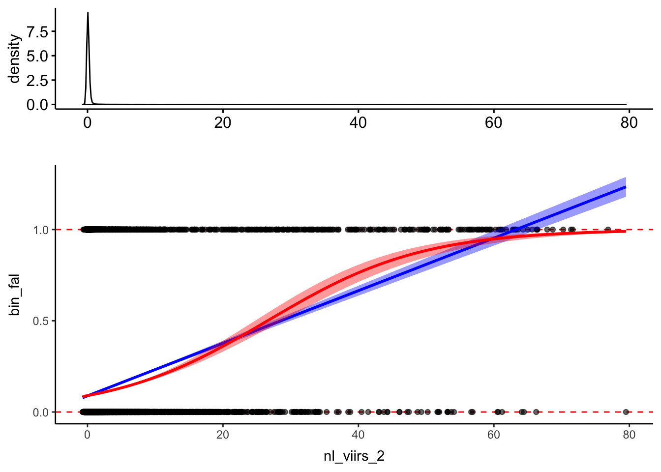

In STATA

xtreg bin_fal nl_viirs_2_s, cl(provincex) fe

xtreg bin_fal nl_viirs_2_s mei_ike_udel, cl(provincex) fe

3.3 Negative Binomial Model

3.3.1 Model vivax

Monthly data

dat %>% ggplot (aes(viv_rate)) +
  geom_histogram() + theme_bw()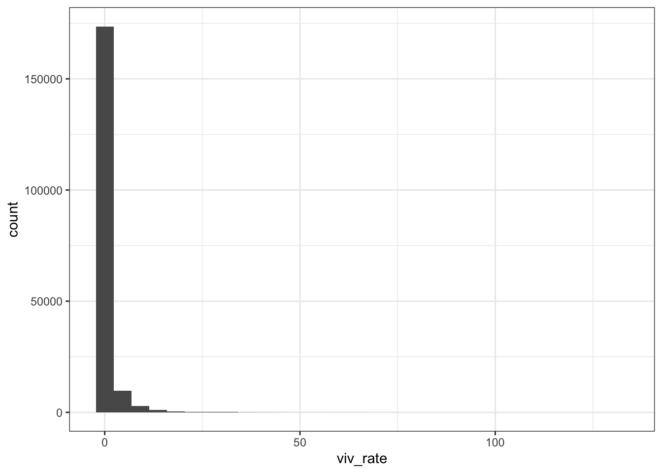

Yearly data

dat_year %>% ggplot (aes(viv_rate)) +
  geom_histogram() + theme_bw()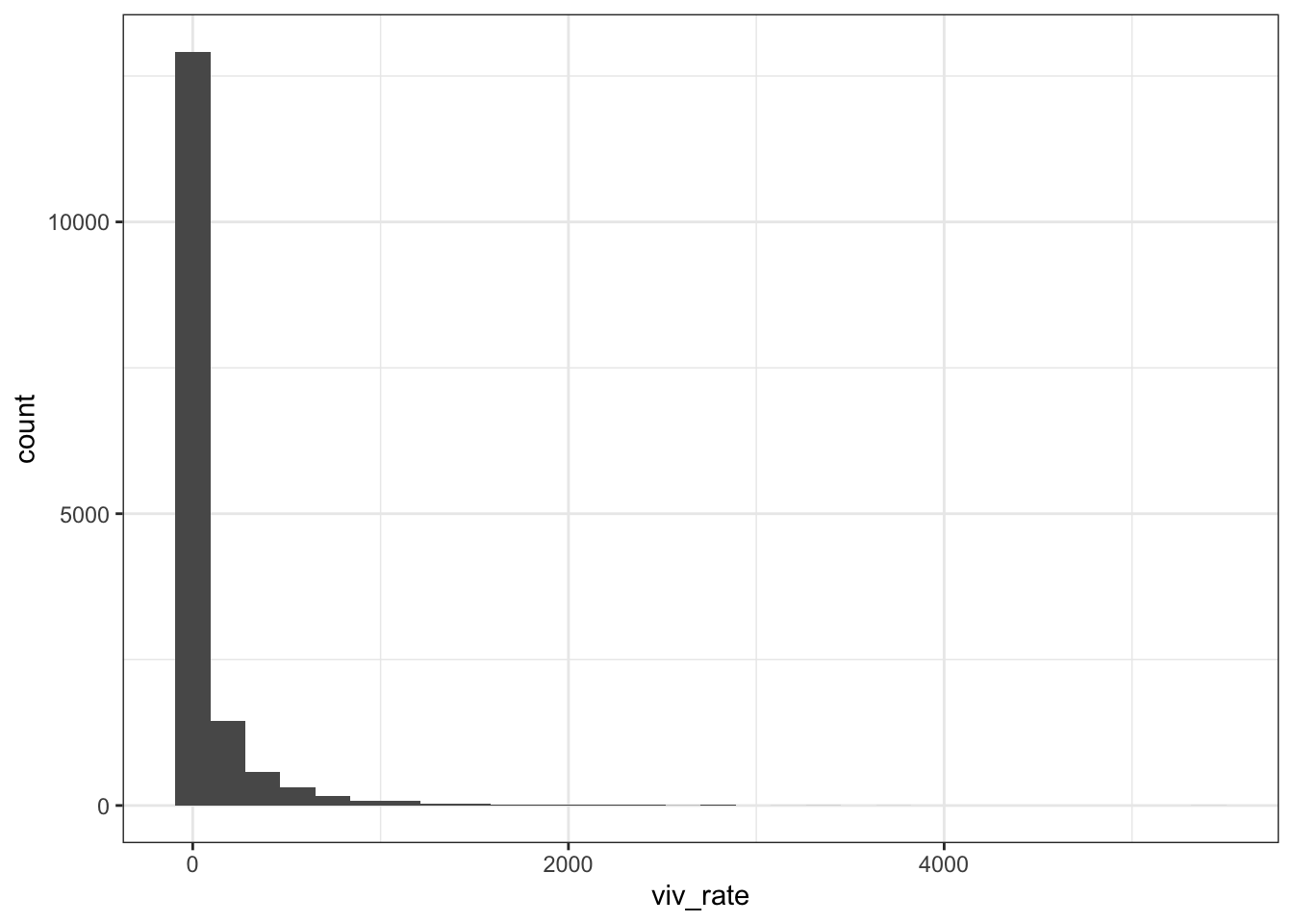

In STATA

xtnbreg viv nl_viirs_2_s, exp(nrohab) fe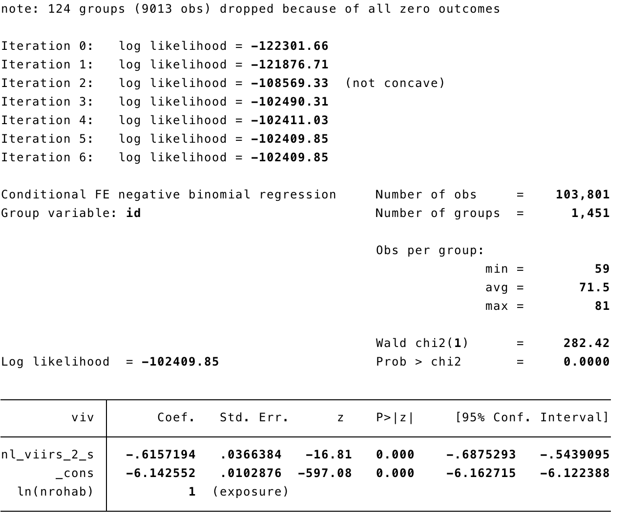

xtnbreg viv nl_viirs_2_s, exp(nrohab) fe eform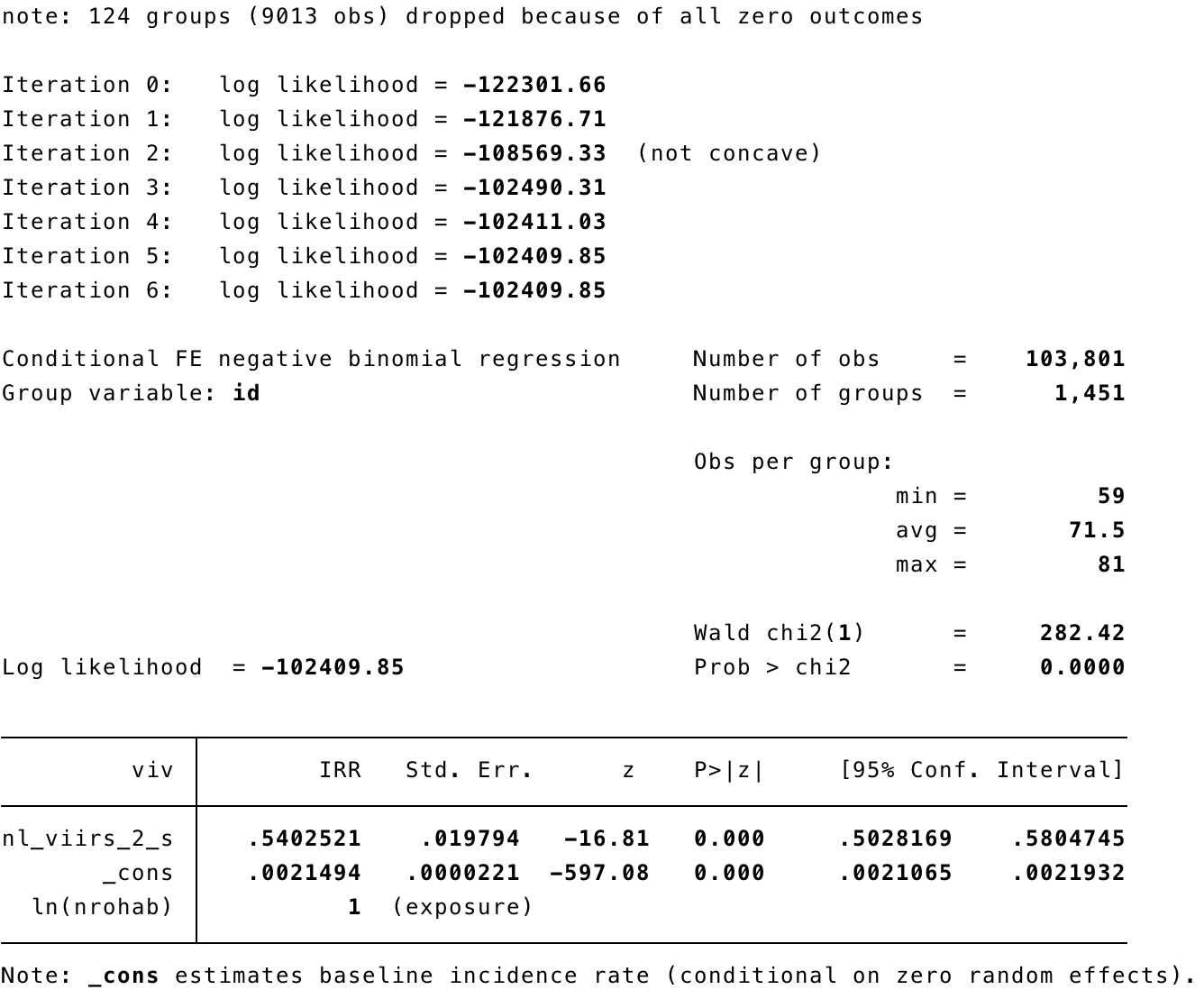

xtnbreg viv nl_viirs_2_s mei_ike_udel, exp(nrohab) fe eform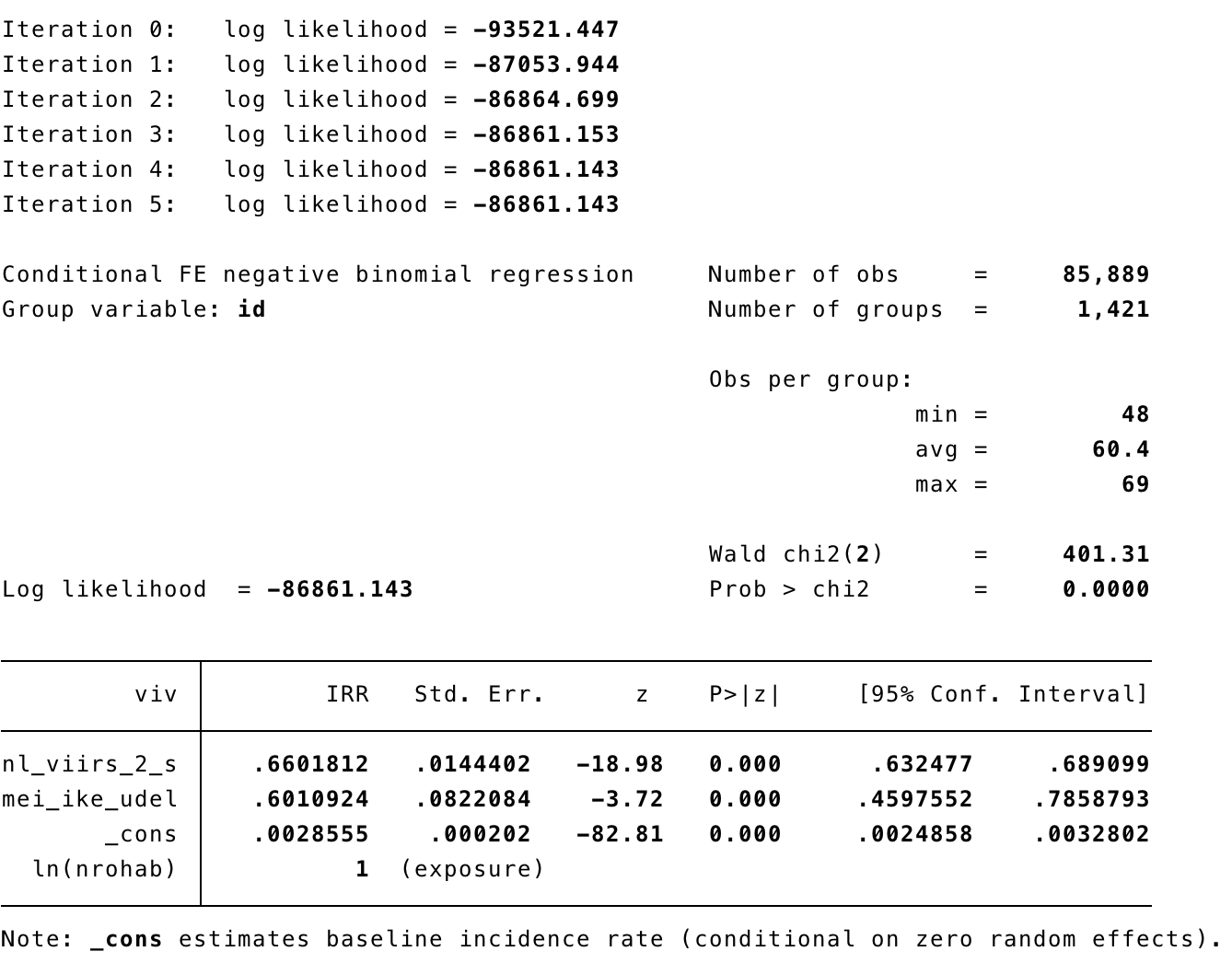

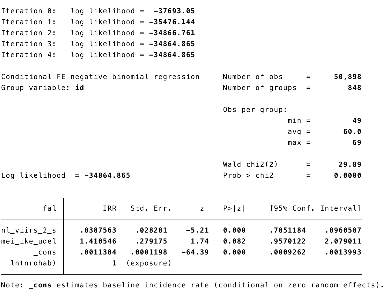
3.3.2 Model falciparum

Monthly data

dat %>% ggplot (aes(fal_rate)) +
  geom_histogram() + theme_bw()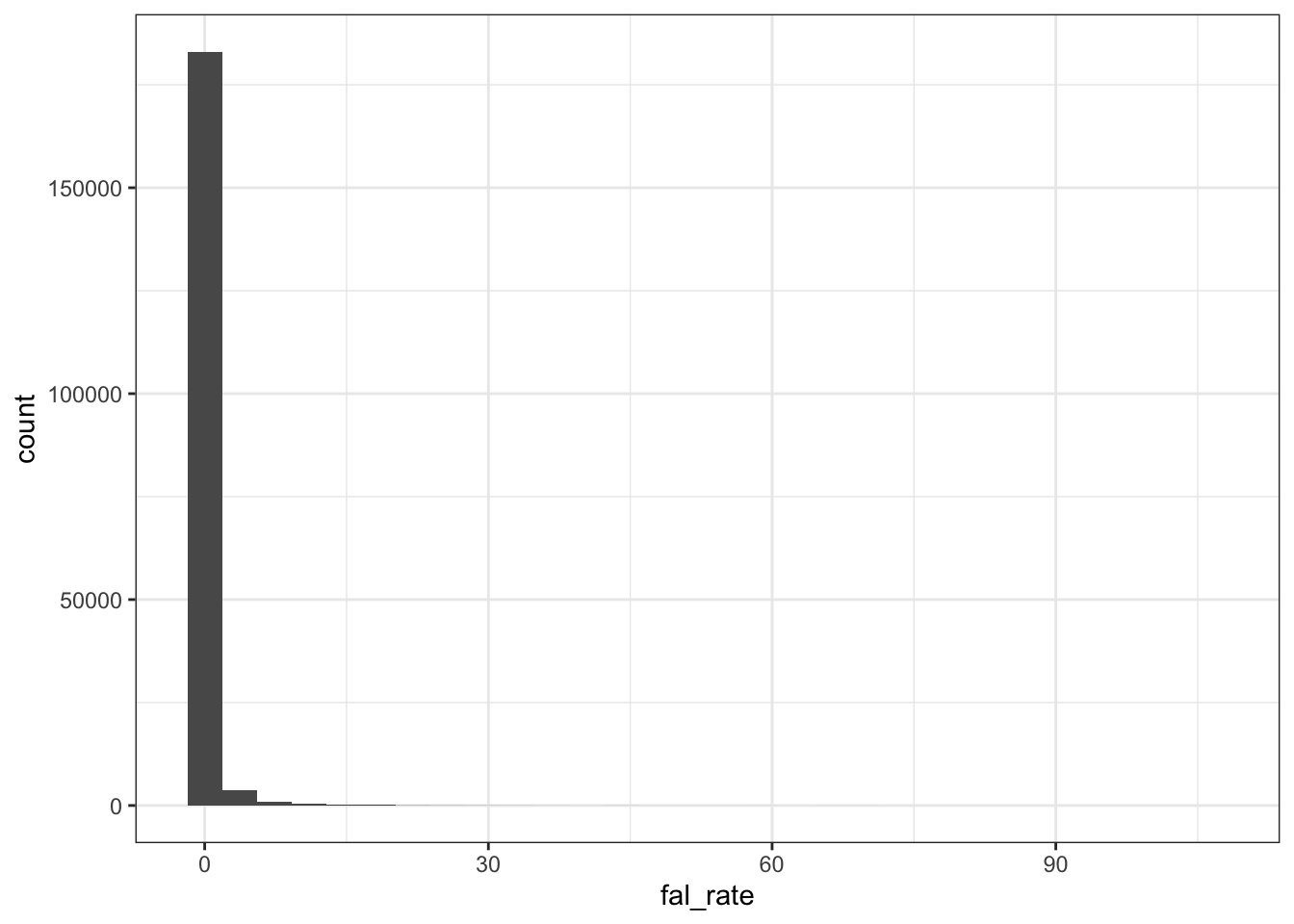

Yearly data

dat_year %>% ggplot (aes(fal_rate)) +
  geom_histogram() + theme_bw()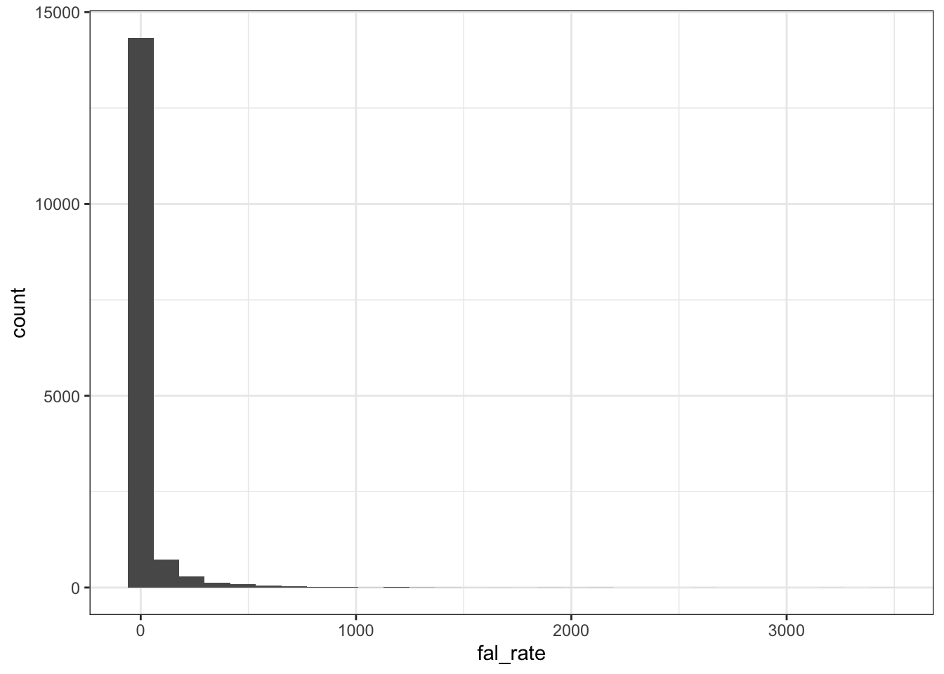

In STATA

xtnbreg fal nl_viirs_2_s, exp(nrohab) fe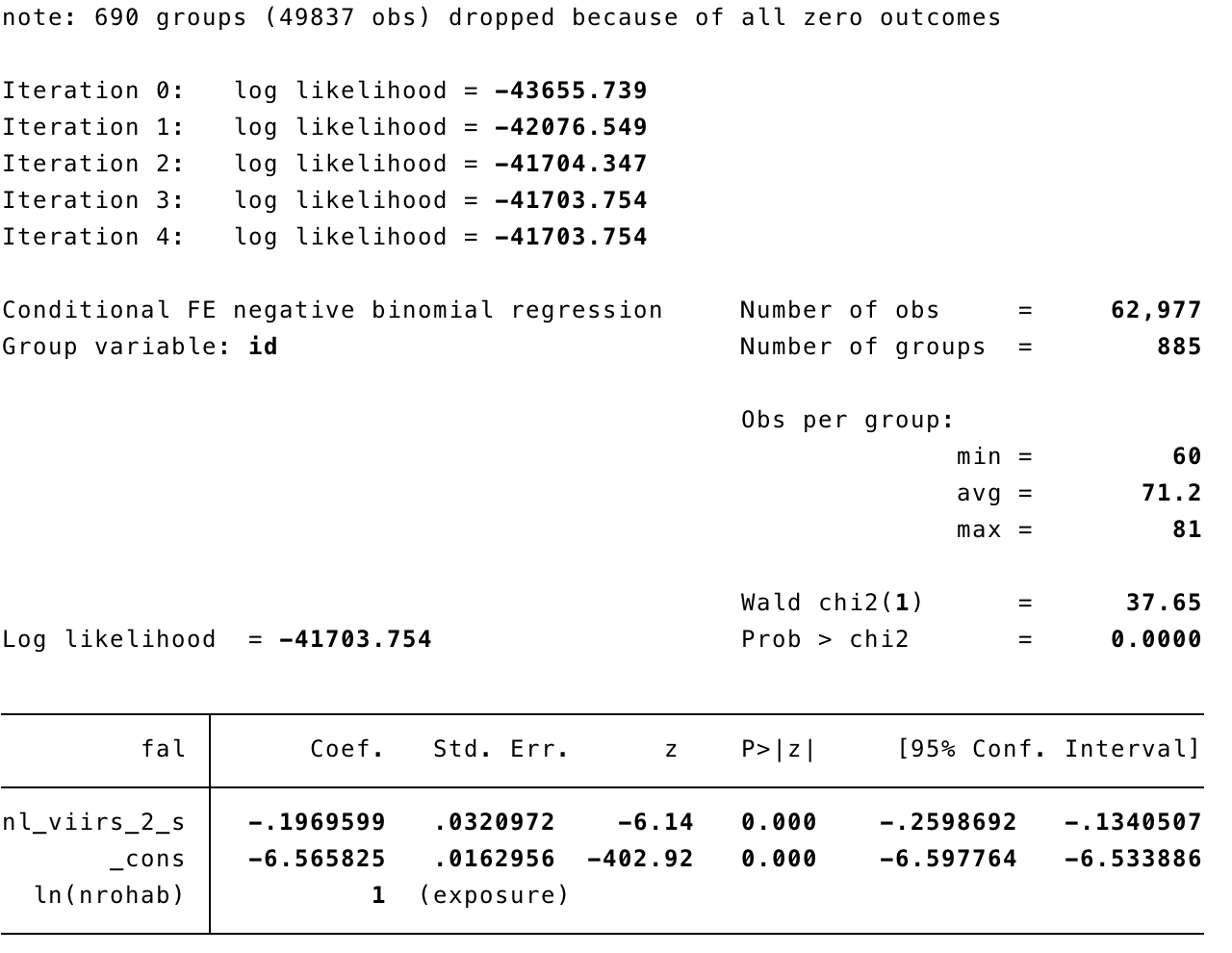

xtnbreg fal nl_viirs_2_s, exp(nrohab) fe eform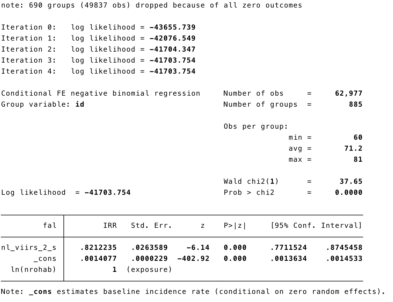

xtnbreg fal nl_viirs_2_s mei_ike_udel, exp(nrohab) fe eform