Chapter 2 Aim1: PREDICTION CAPACITY [Random Effects model]

2.1 Data

rm(list=ls())

library(raster)
library(sf)
library(rasterVis)
library(tidyverse)
library(haven)
library(stringr)
library(scales)
library(cowplot)
library(ggpubr)

dat <- readRDS(file.path(wd, "/dat_NL_MAL.RData")) %>%
  filter(nrohab>20) %>%
  mutate(fal_rate = 100*fal/nrohab,
         viv_rate = 100*viv/nrohab)

dat_year <- dat %>%
  ungroup() %>%
  group_by(year, id_loc) %>%
  filter(nrohab>20) %>%
  summarise(provinc = first(province.x),
            fal = sum(fal),
            viv = sum(viv),
            nrohab = mean(nrohab),
            MEI_ike_udel = mean(MEI_ike_udel),
            nl_viirs_2 = mean(nl_viirs_2, na.rm=T),
            nl_viirs_2_max = max(nl_viirs_2, na.rm=T)) %>%
  mutate(fal_rate = 1000*fal/nrohab,
         viv_rate = 1000*viv/nrohab,
         bin_viv = ifelse(viv>0, 1,0),
         bin_fal = ifelse(fal>0, 1,0)) 

dat_year_2 <- dat_year %>%
  filter(nl_viirs_2_max < quantile(dat_year$nl_viirs_2_max, 0.99),
         !is.na(nl_viirs_2)) %>%
  mutate(nl_viirs_2_max_sq = nl_viirs_2_max^2,
         drop = ifelse(viv>nrohab,1,0),
         drop = ifelse(fal>nrohab,1,drop)) %>%
  ungroup() %>%
  group_by(id_loc) %>%
  mutate(drop2 = max(drop, na.rm = T)) %>%
  filter(drop==0)

db <- readRDS("~/Dropbox/Work/SESYNC/Projects/Malaria/Village Level [Javier]/Analysis/output/data_sf.RData") %>%
  mutate(id2 = row_number())

villages <- db %>%
  dplyr::select(id_loc, id2) %>%
  inner_join(st_set_geometry(db, NULL) %>%
               dplyr::select(id_loc, nrohab, village.x, commune, province.x, uid, id2) %>%
               distinct(id_loc, .keep_all = T), by=c("id_loc", "id2")) %>%
  filter(id_loc!="")

river <- st_read("~/Dropbox/Resources/GIS/Hidro_HDX/rionavegables/Rio_navegables.shp") %>%
  filter(i==1) %>%
  st_transform("+proj=longlat +datum=WGS84 +no_defs")

d <- read_csv("~/Dropbox/Work/SESYNC/Projects/Malaria/Village Level [Javier]/Analysis/output/dist_amazon.csv") %>%
  dplyr::select(id_loc, distance) %>% 
  mutate(distance = distance*111111)

villages <- villages %>%
  inner_join(d, by = "id_loc")

# NOT RUN
a <- dat_year_2 %>%
  distinct(id_loc, .keep_all = T)
rm(a)

2.2 Model

library(lme4)
library(skimr)
library(broom.mixed)

fit1 <- glmer.nb(viv ~ nl_viirs_2_max + (1 + nl_viirs_2_max | id_loc) + offset(log(nrohab)), dat_year_2)

coeff1 <- ranef(fit1) %>%
  augment() %>%
  mutate(sig = ifelse(lb<0 & ub>0,0,1),
         nl_viirs_2_max = estimate,
         id_loc = as.character(level)) 

coeff1_s <- coeff1 %>%
  filter(sig==1 & variable == "nl_viirs_2_max") %>%
  select(id_loc, nl_viirs_2_max)

coeff1 <- coeff1 %>%
  filter(variable == "nl_viirs_2_max") %>%
  select(id_loc, nl_viirs_2_max)

skim(coeff1, nl_viirs_2_max)

fit3 <- glmer.nb(viv ~ nl_viirs_2_max + provinc + (1 + nl_viirs_2_max | id_loc) + offset(log(nrohab)), dat_year_2)

coeff3 <- ranef(fit3) %>%
  augment() %>%
  mutate(sig = ifelse(lb<0 & ub>0,0,1),
         nl_viirs_2_max2 = estimate,
         id_loc = as.character(level)) 

coeff3_s <- coeff3 %>%
  filter(sig==1 & variable == "nl_viirs_2_max") %>%
  select(id_loc, nl_viirs_2_max2)

coeff3 <- coeff3 %>%
  filter(variable == "nl_viirs_2_max") %>%
  select(id_loc, nl_viirs_2_max2)

skim(coeff3, nl_viirs_2_max2)

2.3 Model sumamry

library(jtools)
summ(fit1)

Observations	10629
Dependent variable	viv
Type	Mixed effects generalized linear model
Family	Negative Binomial(0.6838)
Link	log

AIC	51608.00
BIC	51651.63

Fixed Effects
	Est.	S.E.	z val.	p
(Intercept)	-4.05	0.06	-73.40	0.00
nl_viirs_2_max	-0.21	0.11	-1.88	0.06

Random Effects
Group	Parameter	Std. Dev.
id_loc	(Intercept)	1.99
id_loc	nl_viirs_2_max	0.17

Grouping Variables
Group	# groups	ICC
id_loc	1555	0.38

summ(fit3)

Observations	10629
Dependent variable	viv
Type	Mixed effects generalized linear model
Family	Negative Binomial(0.6485)
Link	log

AIC	51330.61
BIC	51425.13

Fixed Effects
	Est.	S.E.	z val.	p
(Intercept)	-5.22	0.14	-36.01	0.00
nl_viirs_2_max	-0.34	0.14	-2.47	0.01
provincDATEM DEL MARA_ON	1.60	0.19	8.38	0.00
provincLORETO	1.95	0.19	10.14	0.00
provincMARISCAL RAMON CASTILLA	1.66	0.21	7.92	0.00
provincMAYNAS	1.55	0.17	9.13	0.00
provincPUTUMAYO	0.50	0.31	1.58	0.11
provincREQUENA	-0.39	0.23	-1.69	0.09
provincUCAYALI	-3.10	0.48	-6.44	0.00

Random Effects
Group	Parameter	Std. Dev.
id_loc	(Intercept)	1.77
id_loc	nl_viirs_2_max	0.46

Grouping Variables
Group	# groups	ICC
id_loc	1555	0.23

2.4 Output

ggplot() +
  geom_density(data = coeff1, aes(nl_viirs_2_max, fill = "viirs"), col = NA, alpha = .7) +
  geom_density(data = coeff3, aes(nl_viirs_2_max2, fill = "viirs + province"), col = NA, alpha = .7) +
  labs(fill = "Model", x = "viirs beta coefficients", y = "Density") +
  scale_y_continuous(expand = c(0, 0)) + 
  scale_fill_manual(values = c("viirs" = "#9AC0CD", "viirs + province" = "#8B475D")) +
  theme_bw()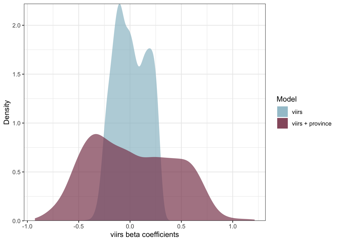

ggplot() +
  geom_density(data = coeff1_s, aes(nl_viirs_2_max, fill = "viirs"), col = NA, alpha = .7) +
  geom_density(data = coeff3_s, aes(nl_viirs_2_max2, fill = "viirs + province"), col = NA, alpha = .7) +
  labs(fill = "Model", x = "viirs beta coefficients", y = "Density") +
  scale_y_continuous(expand = c(0, 0)) + 
  scale_fill_manual(values = c("viirs" = "#9AC0CD", "viirs + province" = "#8B475D")) +
  theme_bw()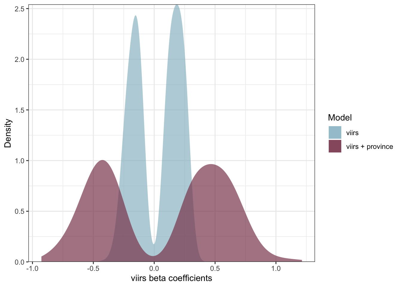

2.4.1 Spatial distribution

coeff3.sf <- villages %>%
  inner_join(coeff3, by="id_loc") %>%
  rename(NOMBPROV = province.x,
         NOMBDIST = commune)

coeff3_s.sf <- villages %>%
  inner_join(coeff3_s, by="id_loc") %>%
  rename(NOMBPROV = province.x,
         NOMBDIST = commune)

area.sf <- st_read("~/Dropbox/Work/Climate and Malaria/Analysis/Data/MapLOR_DIST/MapLOR_DIST.shp")

## Reading layer `MapLOR_DIST' from data source `/Users/gcarrasco/Dropbox/Work/Climate and Malaria/Analysis/Data/MapLOR_DIST/MapLOR_DIST.shp' using driver `ESRI Shapefile'
## Simple feature collection with 49 features and 19 fields
## geometry type:  POLYGON
## dimension:      XY
## bbox:           xmin: -77.82596 ymin: -8.716139 xmax: -69.94904 ymax: -0.03860597
## epsg (SRID):    4326
## proj4string:    +proj=longlat +datum=WGS84 +no_defs

l <- st_read("~/Dropbox/Resources/GIS/per_admbnda_adm1_2018/per_admbnda_adm1_2018.shp") %>%
  filter(ADM1_ES =="Loreto")

## Reading layer `per_admbnda_adm1_2018' from data source `/Users/gcarrasco/Dropbox/Resources/GIS/per_admbnda_adm1_2018/per_admbnda_adm1_2018.shp' using driver `ESRI Shapefile'
## Simple feature collection with 25 features and 7 fields
## geometry type:  MULTIPOLYGON
## dimension:      XY
## bbox:           xmin: -81.32823 ymin: -18.35093 xmax: -68.65228 ymax: -0.03860597
## epsg (SRID):    4326
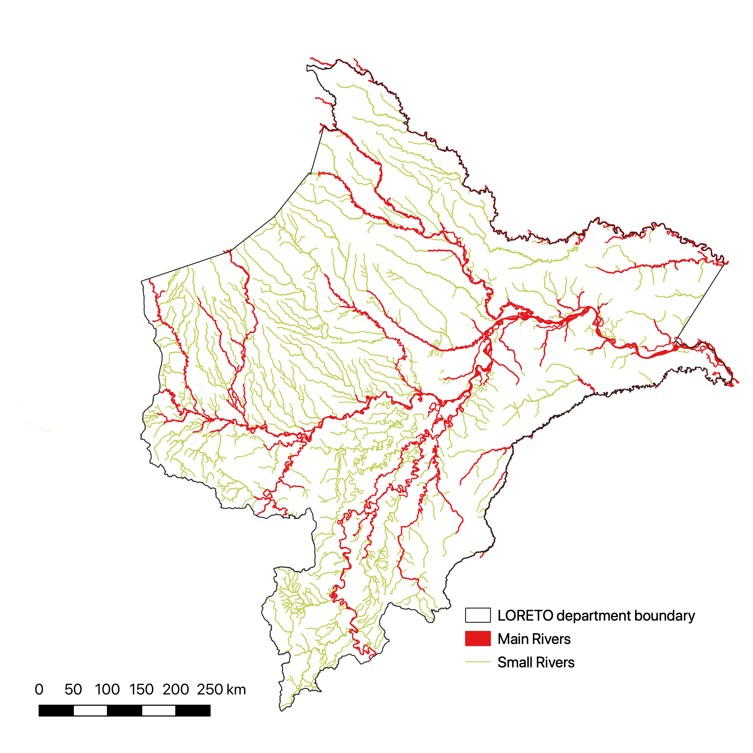
## proj4string:    +proj=longlat +datum=WGS84 +no_defs

#river
bb <- st_bbox(l)
bb[1] <- -77.6
river.l <- st_crop(river,bb)

area.sf_coeff_s <- area.sf %>%
  inner_join(st_set_geometry(coeff3_s.sf, NULL) %>%
               group_by(NOMBDIST) %>%
               summarise(coeff = mean(nl_viirs_2_max2)),
             by = "NOMBDIST")

area.sf_coeff <- area.sf %>%
  inner_join(st_set_geometry(coeff3.sf, NULL) %>%
               group_by(NOMBDIST) %>%
               summarise(coeff = mean(nl_viirs_2_max2)),
             by = "NOMBDIST")

2.5 Figures

2.5.1 Figure post1

ggplot() + 
  geom_sf(data = l, size = 0.5, col = "black") +
  geom_sf(data = river.l, col="#8B1C62", size = 0.3) +
  geom_sf(data = coeff3_s.sf, aes(col=nl_viirs_2_max2, size = nrohab), alpha=.3) +
  scale_color_gradient2(low = "#00688B", mid = "white", high = "#CD3700") +
  labs(color = "viirs RE slope") +
  theme_void() +
  theme(axis.text = element_text(size = 15))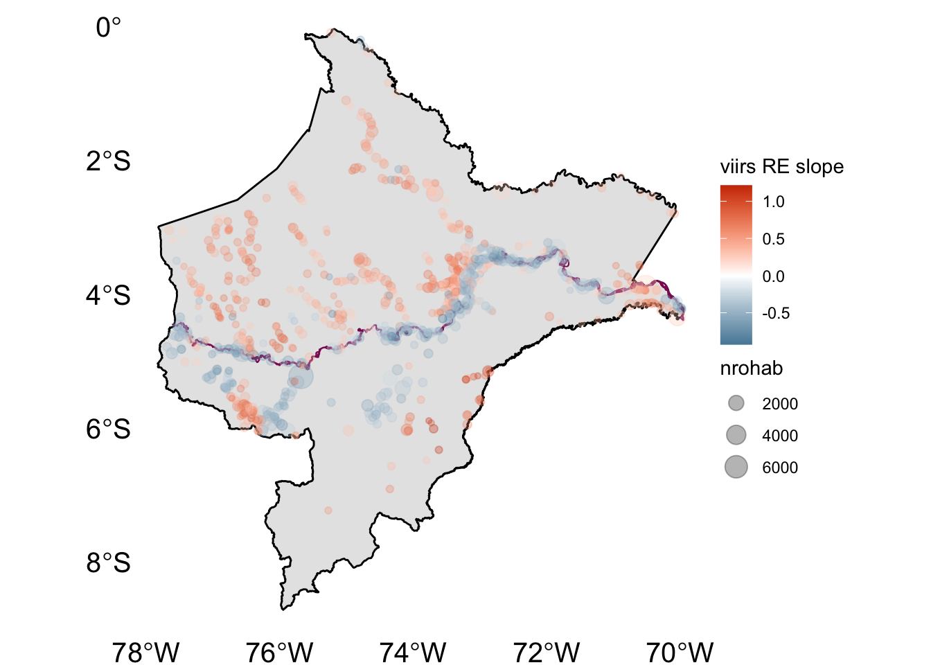

2.5.2 Figure post2

area.sf_top = coeff3_s.sf %>% 
            mutate(low = ifelse(ntile(nl_viirs_2_max2,100)<3,"low","a"),
                   high = ifelse(ntile(nl_viirs_2_max2,100)>98,"high","a"),
                   beta = ifelse(low=="a",high,low)) %>%
            filter(beta!="a")

ggplot() + 
  geom_sf(data = l, fill=NA, size = 0.5, col = "black") +
  geom_sf(data = river.l, col="#8B1C62", size = 0.3) +
  geom_sf(data = area.sf_top,
          aes(col=beta), size = 2, alpha=.5) +
  labs(color = "viirs RE slope") +
  theme_void() +
  theme(axis.text = element_text(size = 15))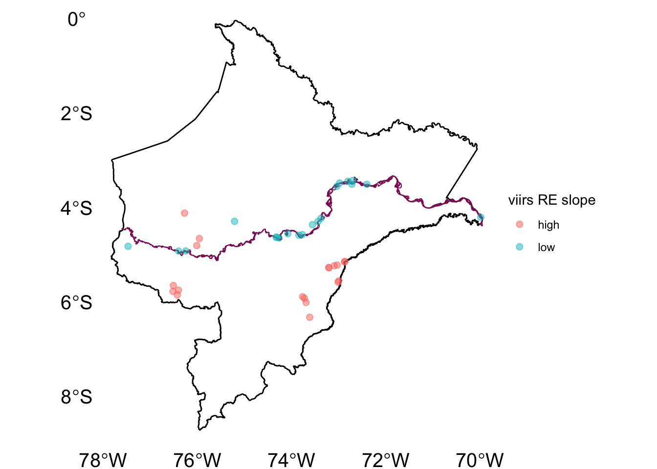

2.5.3 Figure post3 [skip]

# area.sf_top %>%
#   filter(beta=="low") %>%
#   st_set_geometry(NULL) %>%
#   dplyr::select(id_loc) %>%
#   left_join(dat_year_2, by = "id_loc") %>%
#   ggplot(aes(x = year, group = id_loc)) +
#   geom_line(aes(y = viv_rate, col = "viv rate")) + 
#   geom_line(aes(y = nl_viirs_2_max*10, col = "viirs")) + 
#   scale_color_manual(values = c("viv rate" = "black", "viirs" = "red")) +
#   labs(col = "var", x = "year", y = "", title = "villages with most negative betas") +
#   scale_y_continuous("viv rate", sec.axis = sec_axis(~ . / 10, name = "viirs")) +
#   facet_wrap(.~id_loc, scales = "free_y")
# 
# area.sf_top %>%
#   filter(beta=="high") %>%
#   st_set_geometry(NULL) %>%
#   dplyr::select(id_loc) %>%
#   left_join(dat_year_2, by = "id_loc") %>%
#   ggplot(aes(x = year, group = id_loc)) +
#   geom_line(aes(y = viv_rate, col = "viv rate")) + 
#   geom_line(aes(y = nl_viirs_2_max*3000, col = "viirs")) + 
#   scale_color_manual(values = c("viv rate" = "black", "viirs" = "red")) +
#   labs(col = "var", x = "year", y = "", title = "villages with most positive betas") +
#   scale_y_continuous("viv rate", sec.axis = sec_axis(~ . / 3000, name = "viirs")) +
#   facet_wrap(.~id_loc, scales = "free_y")

2.5.4 Figure post4 [Figure 2]

(map <- area.sf_coeff_s %>% #mutate(NOMBDIST2 = factor(NOMBDIST, levels=unique(NOMBDIST[order(NOMBPROV)]), ordered=TRUE)) %>%
  ggplot() + 
  geom_sf(aes(fill=coeff), size = 0.5, col = NA) +
  geom_sf(data = l, fill=NA, size = 0.5, col = "black") +
  geom_sf(data = river.l, aes(color="Amazon River"), size = 0.3, show.legend = "line") +
  scale_fill_gradient2(low = "#00688B", mid = "white", high = "#CD3700") +
  scale_color_manual(values = "#8B1C62", name = "") +
  labs(fill = "Mean Coeff") +
  theme_bw() +
  theme(axis.text = element_text(size = 10),
        legend.position = "bottom"))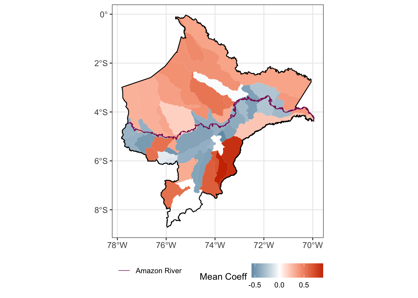

library(cowplot)
f2 <- plot_grid(map, labels = c("A"))

#ggsave(f2, filename = "./_out/f2.png", width = 5, height = 6, dpi = 300)

library(ggExtra)

a <- dat %>%
  filter(!is.na(nl_viirs_2)) %>%
  st_set_geometry(NULL) %>%
  group_by(id_loc) %>%
  summarise(nl_viirs_2 = first(nl_viirs_2)) %>%
  mutate(nl_viirs_2 = ifelse(nl_viirs_2<0,0,nl_viirs_2))

b <- coeff3.sf %>% #cambiar
  inner_join(a, by= "id_loc") %>%
  inner_join(area.sf_coeff %>% # cambiar
               st_set_geometry(NULL) %>%
               mutate(dist = ifelse(coeff<0, "main river", "small river")) %>%
               dplyr::select(NOMBDIST, dist), 
             by= "NOMBDIST")

2.5.5 VIIRS baseline vs. beta

b %>%
  ggplot(aes(x=nl_viirs_2, y=nl_viirs_2_max2)) +
  geom_point(alpha=.3) +
  scale_x_continuous(trans="log10", labels = scales::comma_format()) +
  labs(x = "viirs baseline", y = "viirs beta") + 
  geom_smooth(method = "loess", col="red", fill="red") +
  stat_smooth(method = "lm", formula = y ~ poly(x, 2), col="blue", fill="blue") +
  theme_bw()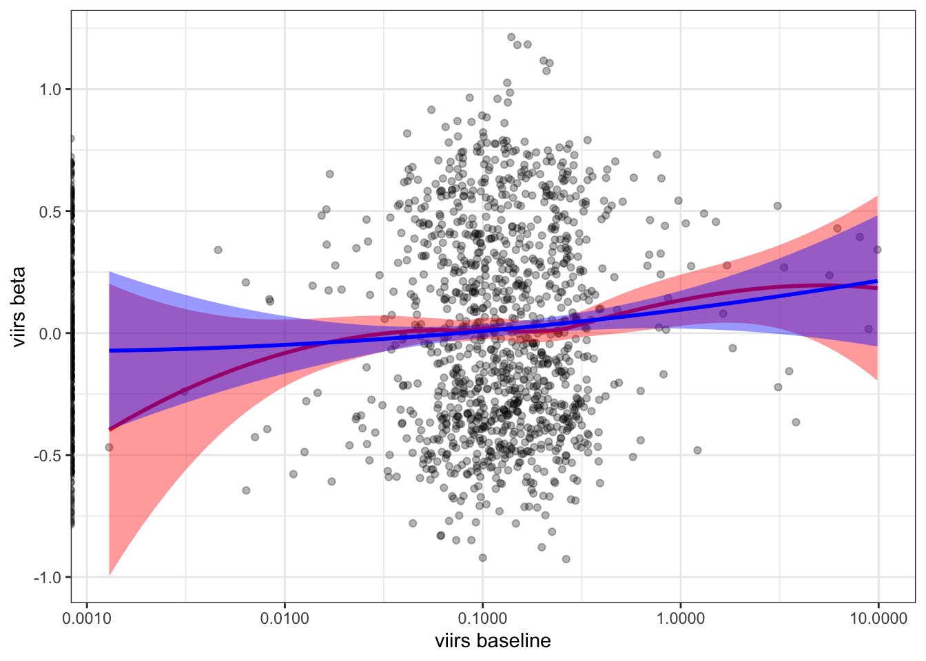

2.5.6 Distance to Amazon vs. beta [Fig 3a]

f3a.p <- b %>%
  ggplot(aes(x=distance, y=nl_viirs_2_max2)) +
  geom_point(alpha=.3, shape = 3) +
  scale_x_continuous(trans="log10", labels = scales::comma_format()) +
  labs(x = "Distance to Amazon River (m)", y = "VIIRS beta") + 
  #geom_smooth(method = "loess", col="red", fill="red") +
  stat_smooth(method = "lm", formula = y ~ poly(x, 2), col="#FDE725FF", fill="#FDE725FF") +
  theme_bw()

f3a <- ggMarginal(f3a.p, xparams = list(fill = "#481568FF", col = "#440154FF", alpha=.3), #margins = 'x',
           yparams = list(fill = "#29AF7FFF", col = "#20A386FF", alpha=.3))

f3a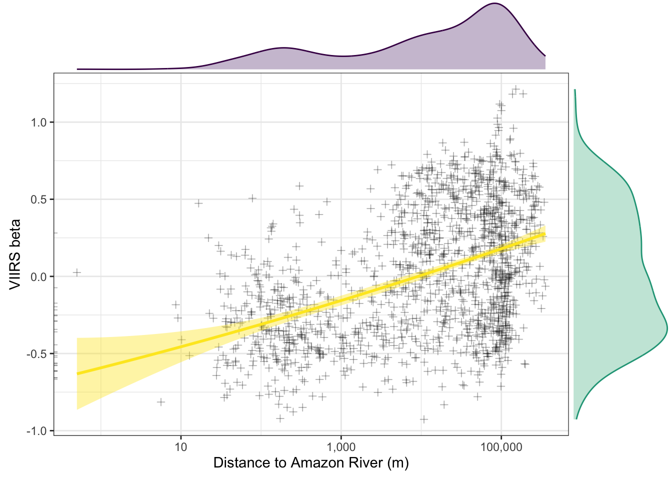

2.5.7 Distance to Amazon vs. VIIRS baseline

b %>%
  ggplot(aes(x=distance, y=nl_viirs_2)) +
  geom_point(alpha=.3) +
  scale_x_continuous(trans="log10", labels = scales::comma_format()) +
  scale_y_continuous(trans="log10", labels = scales::comma_format()) +
  labs(x = "distance to Amazon river", y = "viirs baseline") + 
  geom_smooth(method = "loess", col="red", fill="red") +
  stat_smooth(method = "lm", formula = y ~ poly(x, 2), col="blue", fill="blue") +
  theme_bw()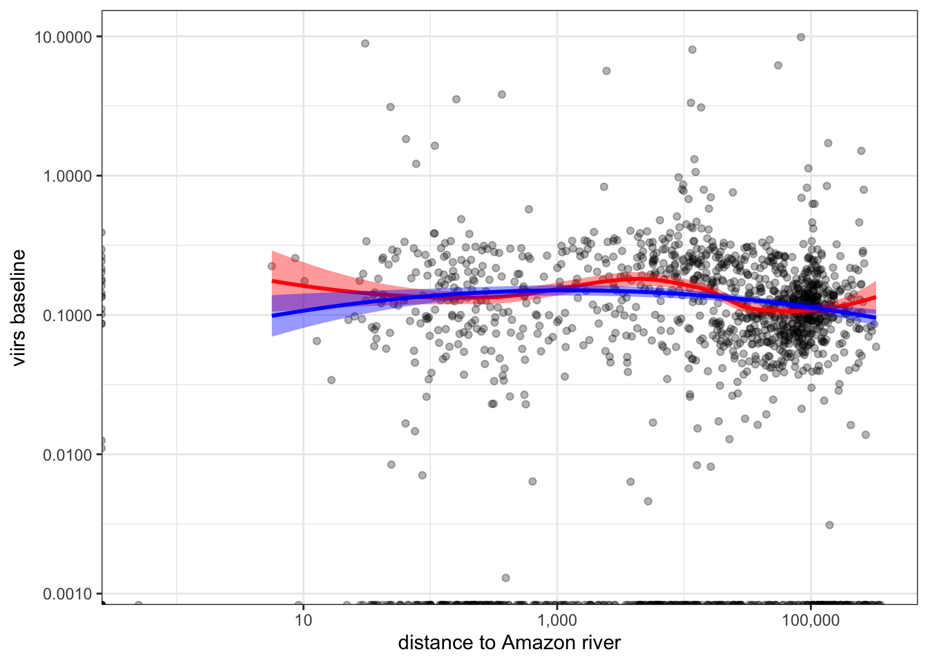

2.5.8 Popualtion vs. beta [Fig 3b]

f3b.p <- b %>%
  ggplot(aes(x=nrohab, y=nl_viirs_2_max2)) +
  geom_point(alpha=.3, shape = 3) +
  scale_x_continuous(trans="log10", labels = scales::comma_format()) +
  labs(x = "Population (hab.)", y = "VIIRS beta") + 
  #geom_smooth(method = "loess", col="red", fill="red") +
  stat_smooth(method = "lm", formula = y ~ poly(x, 2), col="#FDE725FF", fill="#FDE725FF") +
  theme_bw()

f3b <- ggMarginal(f3b.p, xparams = list(fill = "#481568FF", col = "#440154FF", alpha=.3), 
           yparams = list(fill = "#29AF7FFF", col = "#20A386FF", alpha=.3))

library(cowplot)
f3 <- plot_grid(f3a, f3b, labels = c("A","B"))
f3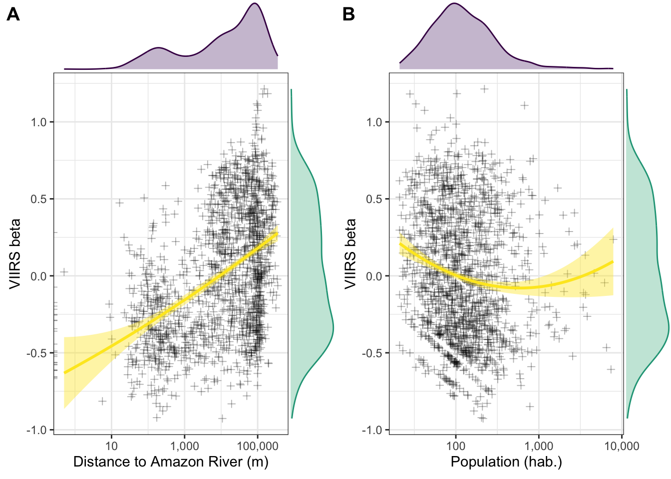

#ggsave2(f3, filename = "./_out/f3.png", width = 12, height = 7, dpi = 300)

2.5.9 Popualtion vs. VIIRS baseline

b %>%
  ggplot(aes(x=nrohab, y=nl_viirs_2)) +
  geom_point(alpha=.3) +
  scale_x_continuous(trans="log10", labels = scales::comma_format()) +
  scale_y_continuous(trans="log10", labels = scales::comma_format()) +
  labs(x = "Population", y = "viirs baseline") + 
  geom_smooth(method = "loess", col="red", fill="red") +
  stat_smooth(method = "lm", formula = y ~ poly(x, 2), col="blue", fill="blue") +
  theme_bw()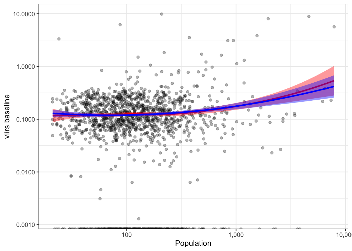

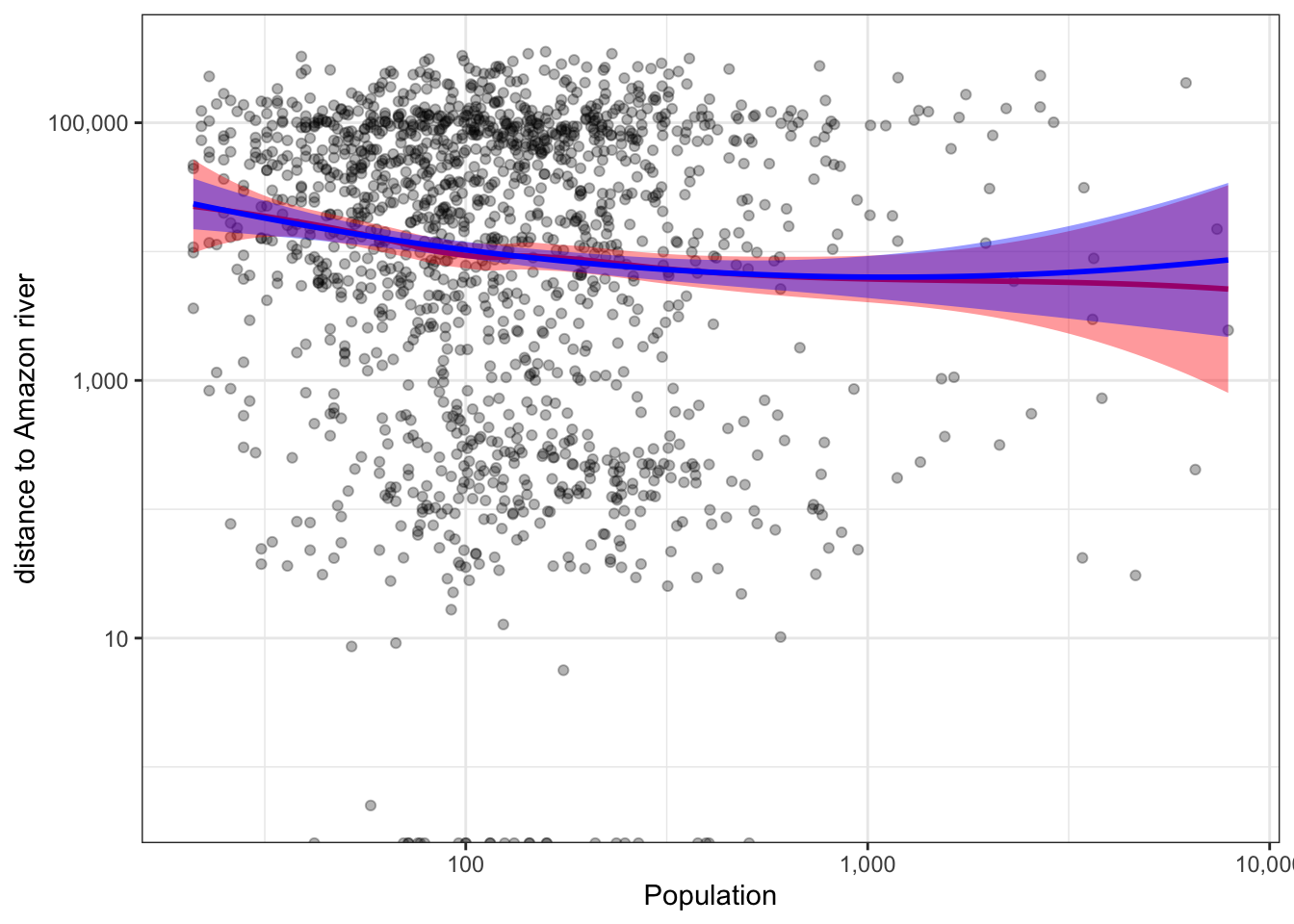
2.5.10 Popualtion vs. Distance to Amazon

b %>%
  ggplot(aes(x=nrohab, y=distance)) +
  geom_point(alpha=.3) +
  scale_x_continuous(trans="log10", labels = scales::comma_format()) +
  scale_y_continuous(trans="log10", labels = scales::comma_format()) +
  labs(x = "Population", y = "distance to Amazon river") + 
  geom_smooth(method = "loess", col="red", fill="red") +
  stat_smooth(method = "lm", formula = y ~ poly(x, 2), col="blue", fill="blue") +
  theme_bw()