Chapter 2 DEMO
2.1 Init
# install.packages("rEDM")

library(tidyverse)
library(lubridate)
library(rEDM)
2.2 Example 1
From: https://github.com/SugiharaLab/rEDM/blob/master/vignettes/rEDM-tutorial.pdf
2.2.1 Sardine-Anchovie-Temperature problem
cmap <- CCM(dataFrame = sardine_anchovy_sst, E = 3, Tp = 0, columns = "anchovy",
            target = "np_sst", libSizes = "10 70 5", sample = 100, showPlot = TRUE)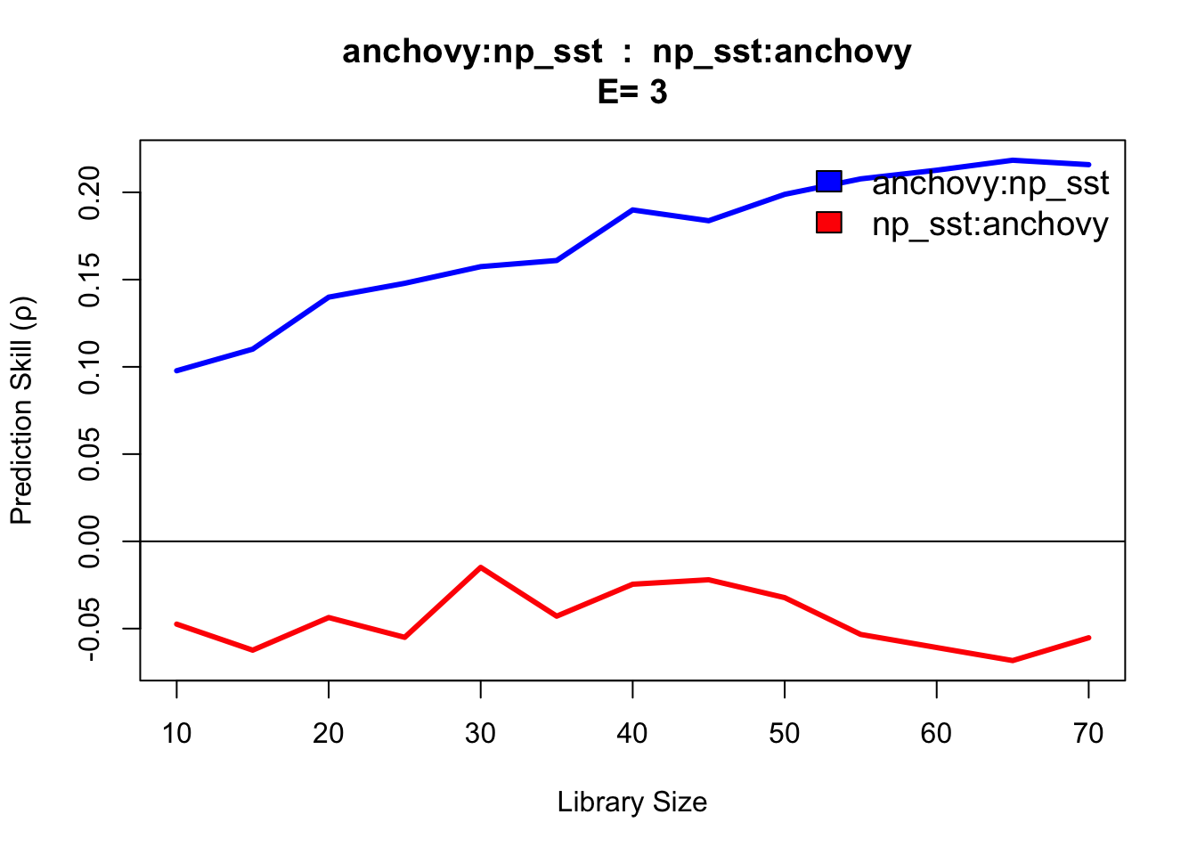
2.2.2 Real data Example
head(Thrips, 2)## Year Month Thrips_imaginis maxT_degC Rain_mm Season
## 1 1932 4 4.5 19.2 140.1 -0.500
## 2 1932 5 23.4 19.1 53.7 -0.866Thrips %>%
gather(var, val, Thrips_imaginis:Season) %>%
mutate(date = ymd(paste(Year, Month, "1", sep = "/"))) %>%
ggplot(aes(x = date, y = val, col = var)) +
geom_line() +
guides(col = F) +
facet_wrap(.~var, ncol = 1, scales = "free") +
theme_bw()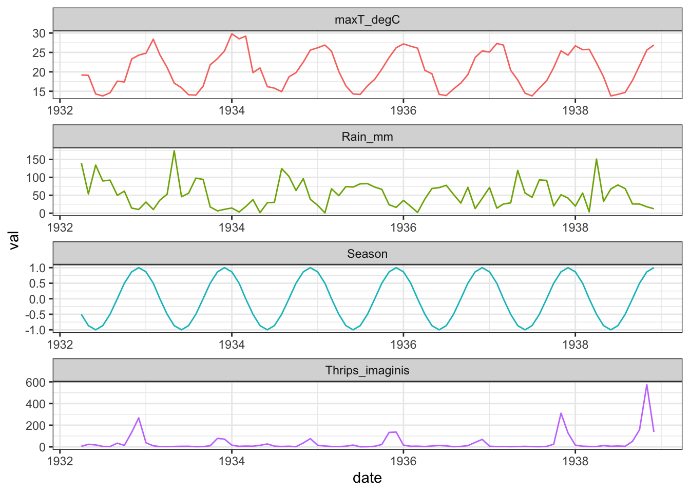
2.2.2.1 Univariate Analysis
We first examine the dependence of simplex predictability on the embedding dimension.
rho_E <- EmbedDimension(dataFrame = Thrips, columns = "Thrips_imaginis",
                        target = "Thrips_imaginis", lib = "1 72",
                        pred = "1 72", showPlot = TRUE)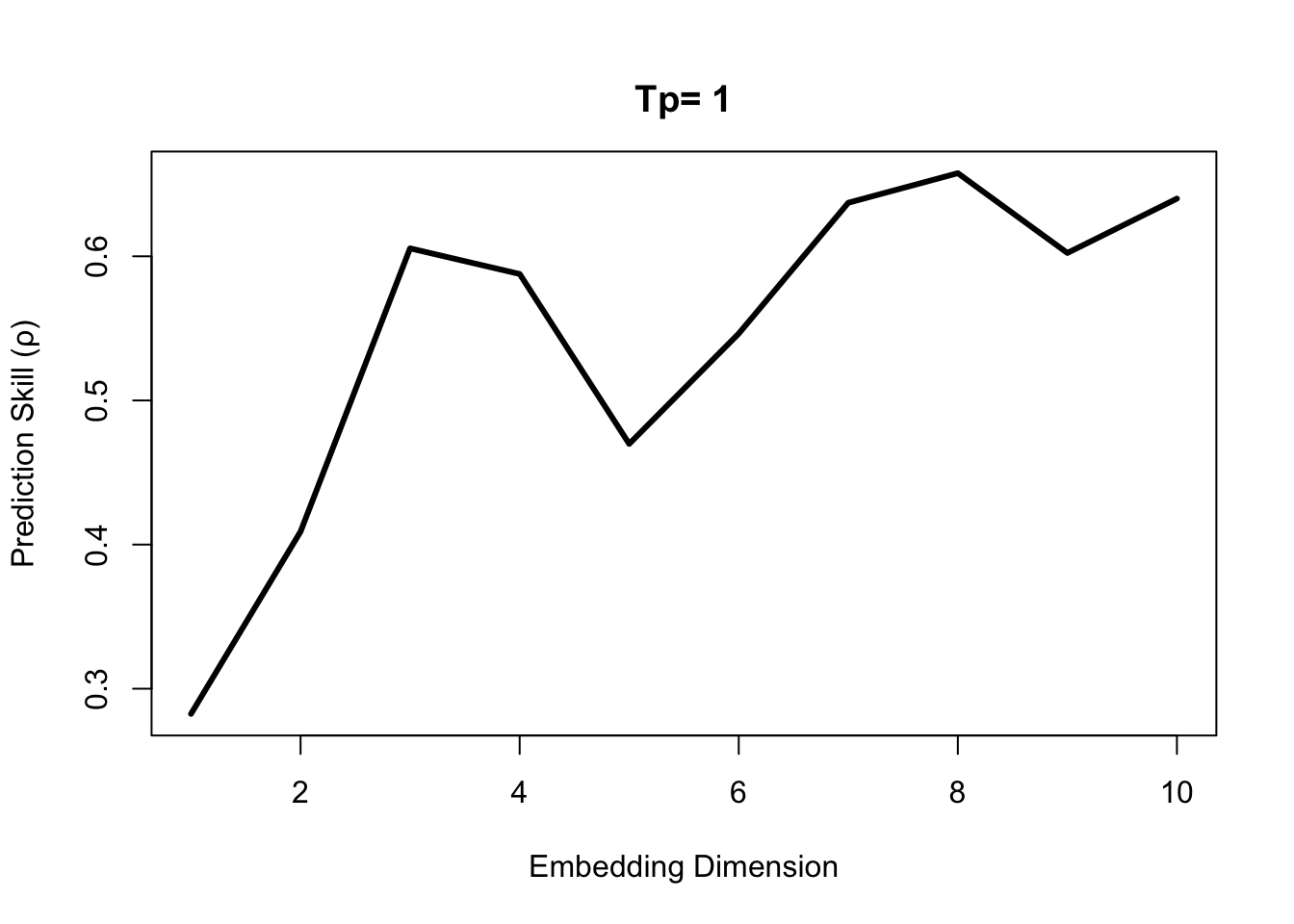
While there is an initial peak in the simplex prediction at E = 3, the global maximum is at E = 8. This suggests that both E = 3 and E = 8 are practical embedding dimensions, although E = 8 is preferrable with a higher predictive skill.
To test for nonlinearity we use the S-map PredictNonlinear() function.
E = 8
rho_theta_e3 = PredictNonlinear(dataFrame = Thrips, columns = "Thrips_imaginis",
                                target = "Thrips_imaginis", lib = "1 73",
                                pred = "1 73", E = E)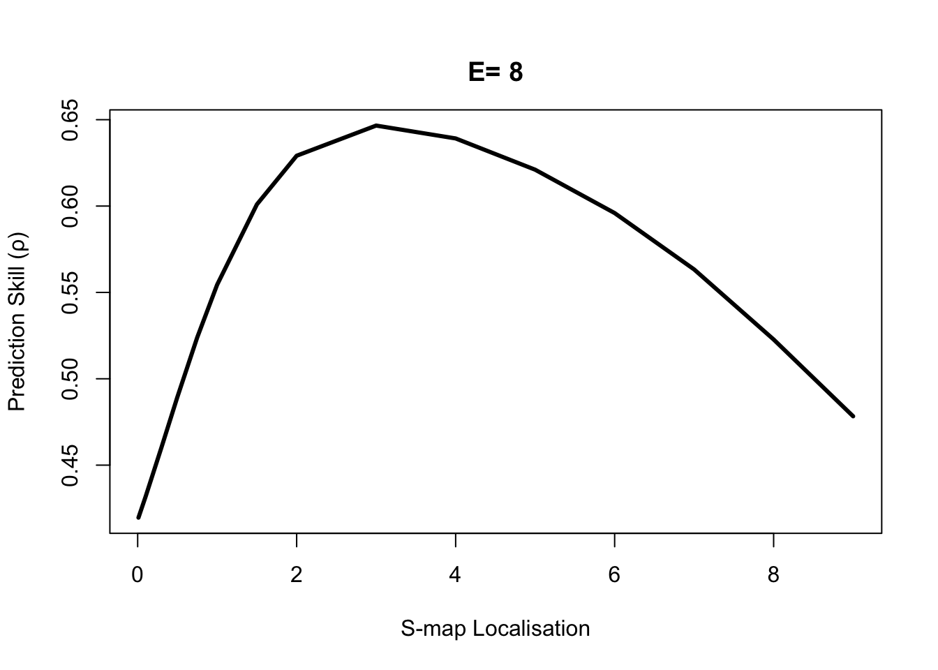
2.2.2.2 Seasonal Drivers
Recall that there is a two-part criterion for CCM to be a rigorous test of causality:
- The cross map prediction skill is statistically significant when using the full time series as the library.
- Cross map prediction demonstrates convergence, i.e. prediction skill increases as more of the time series is used for the library and the reconstructed attractor becomes more dense.
For an initial summary, we first compute the cross map skill (measured with Pearsons ρ) for each variable pair. Note that CCM() computes the cross map in both “directions.”
vars = colnames(Thrips[3:6])
var_pairs = combn(vars, 2) # Combinations of vars, 2 at a time
libSize = paste(NROW(Thrips) - E, NROW(Thrips) - E, 10, collapse = " ")

ccm_matrix = array(NA, dim = c(length(vars), length(vars)), dimnames = list(vars,vars))

for (i in 1:ncol(var_pairs)) {
  ccm_out = CCM(dataFrame = Thrips, columns = var_pairs[1, i], target = var_pairs[2,i],
                libSizes = libSize, Tp = 0, E = E, sample = 100)
  outVars = names(ccm_out)
  var_out = unlist(strsplit(outVars[2], ":"))
  ccm_matrix[var_out[2], var_out[1]] = ccm_out[1, 2]
  var_out = unlist(strsplit(outVars[3], ":"))
  ccm_matrix[var_out[2], var_out[1]] = ccm_out[1, 3]
}

corr_matrix <- array(NA, dim = c(length(vars), length(vars)), dimnames = list(vars, vars))

for (ccm_from in vars) {
  for (ccm_to in vars[vars != ccm_from]) {
    ccf_out <- ccf(Thrips[, ccm_from], Thrips[, ccm_to], type = "correlation",
                   lag.max = 6, plot = FALSE)$acf
    corr_matrix[ccm_from, ccm_to] <- max(abs(ccf_out))
    }
}

ccm_matrix
## Thrips_imaginis maxT_degC Rain_mm Season
## Thrips_imaginis NA 0.6049056 0.4266679 0.5612276
## maxT_degC 0.9223942 NA 0.8215163 0.9625004
## Rain_mm 0.5104673 0.4624375 NA 0.3927441
## Season 0.9545514 0.9918051 0.7773461 NAcorr_matrix## Thrips_imaginis maxT_degC Rain_mm Season
## Thrips_imaginis NA 0.4489876 0.2668395 0.4488334
## maxT_degC 0.4489876 NA 0.5949077 0.9452625
## Rain_mm 0.2668395 0.5949077 NA 0.5332935
## Season 0.4488334 0.9452625 0.5332935 NAWe can see that the cross map strengths are not symmetric. In general CCM(X1 : X2) != CCM(X2 : X1). We also notice that the cross map and correlation between temperature and the seasonal indicator are high, with the cross map results suggesting that the seasonal variable can almost perfectly recover the temperature, ρ = 0.9919. This makes interpretation more complicated, because we have to consider the possibility that cross mapping is simply identifying the shared seasonality between two time series. In other words, cross mapping between temperature and any variable with a seasonal cycle, might suggest an interaction even if there is no actual causal mechanism.
2.2.2.3 Convergent Cross-Mapping
{
  thrips_xmap_maxT <- CCM(dataFrame = Thrips, E = E, Tp = 0, columns = "Thrips_imaginis",
                        target = "maxT_degC", libSizes = "13 73 3", sample = 300, showPlot = TRUE)
  abline(h = corr_matrix["Thrips_imaginis", "maxT_degC"], col = "black", lty = 2)
}


{
  thrips_xmap_maxT <- CCM(dataFrame = Thrips, E = E, Tp = 0, columns = "Thrips_imaginis",
                          target = "Rain_mm", libSizes = "13 73 3", sample = 300, showPlot = TRUE)
  abline(h = corr_matrix["Thrips_imaginis", "Rain_mm"], col = "black", lty = 2)
}

{
  thrips_xmap_maxT <- CCM(dataFrame = Thrips, E = E, Tp = 0, columns = "Thrips_imaginis",
                          target = "Season", libSizes = "13 73 3", sample = 300, showPlot = TRUE)
  abline(h = corr_matrix["Thrips_imaginis", "Season"], col = "black", lty = 2)
}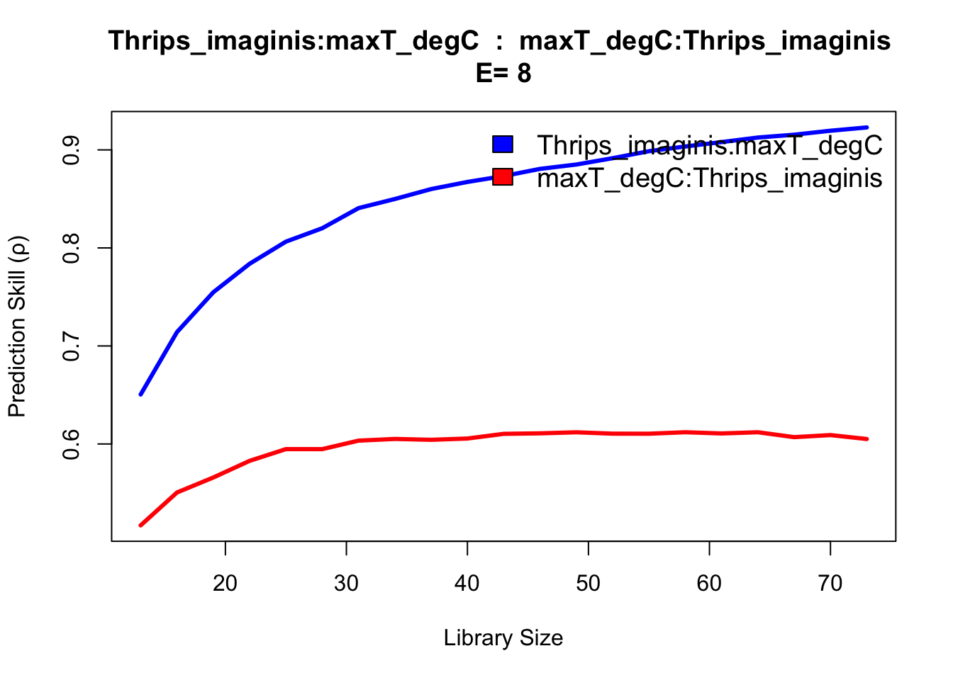
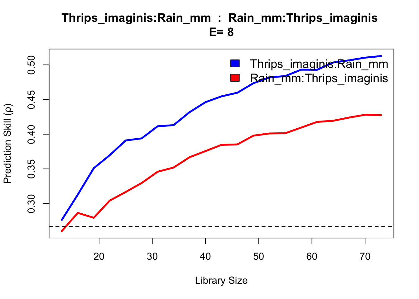
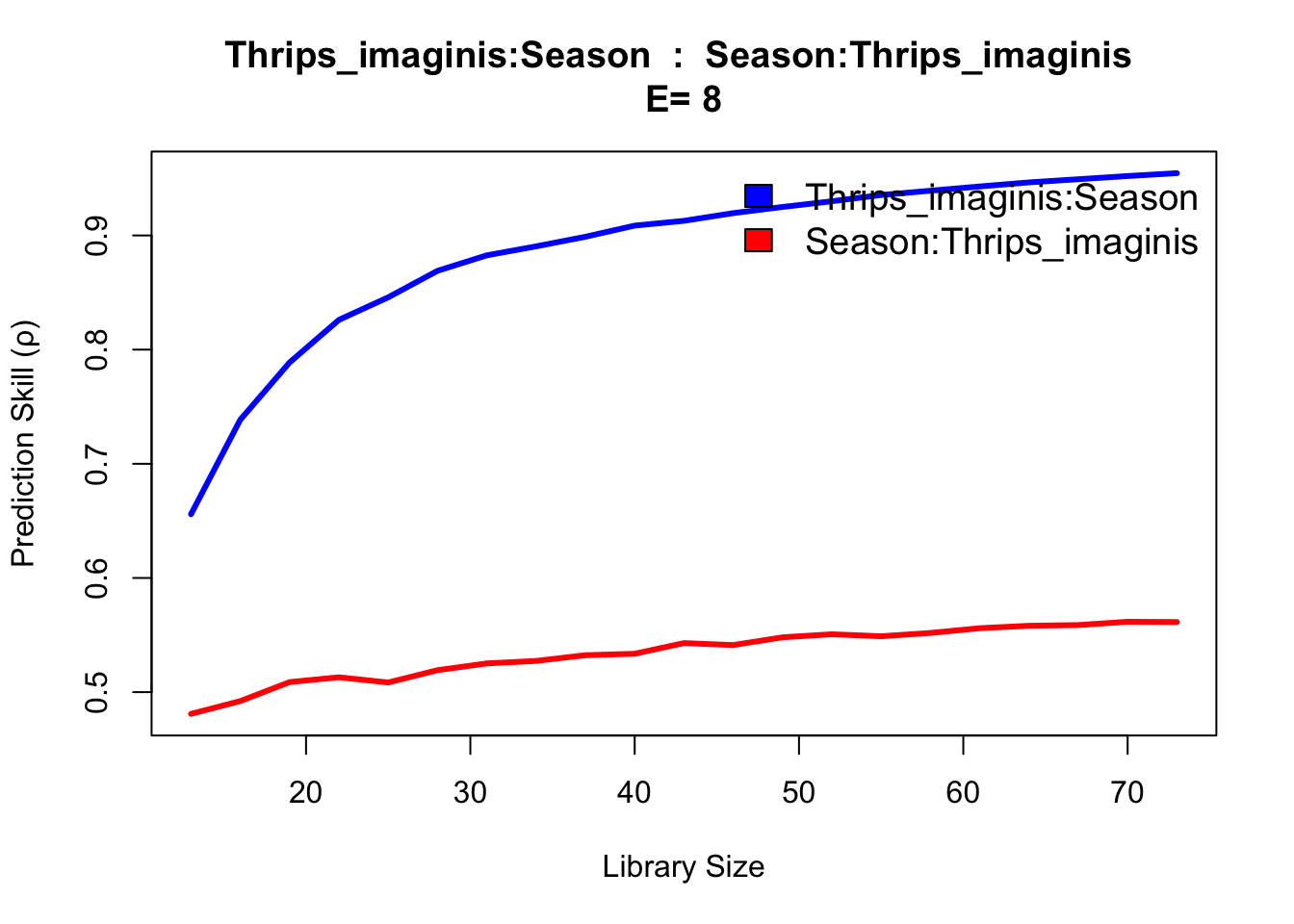
The results show evidence of convergence for Thrips cross mapping to temperature and season variables, with the ρ at maximum library size L significantly exceeding linear correlation. The rain variable does not indicate a substantially different cross map interaction, appearing confounded as to causal influence.
In addition, we are still left with the conundrum that temperature and to a lesser extent, rainfall, are easily predicted from the seasonal cycle, and so we cannot immediately ignore the possibility that the cross map results are an artifact of shared seasonal forcing.
To reframe, we wish to reject the null hypothesis that the level of cross mapping we obtain for maxT_degC and Rain_mm can be solely explained by shared seasonality. This hypothesis can be tested using randomization tests based on surrogate data. The idea here is to generate surrogate time series with the same level of shared seasonality. Cross mapping between the real time series and these surrogates thus generates a null distribution for ρ, against which the actual cross map ρ value can be compared.
2.2.2.4 Seasonal Surrogate Test
# Create matrix with temperature and rain surrogates (1000 time series vectors)
surr_maxT = SurrogateData(Thrips$maxT_degC, method = "seasonal", T_period = 12, num_surr = 1000,
                          alpha = 3)
surr_rain = SurrogateData(Thrips$Rain_mm, method = "seasonal", T_period = 12, num_surr = 1000,
                          alpha = 3)

# Rain cannot be negative
surr_rain = apply(surr_rain, 2, function(x) {
  i = which(x < 0)
  x[i] = 0
  x
  })

# data.frame to hold CCM rho values between Thrips abundance and variable
rho_surr <- data.frame(maxT = numeric(1000), Rain = numeric(1000))

# data.frames with time, Thrips, and 1000 surrogate climate variables for CCM()
maxT_data = as.data.frame(cbind(seq(1:nrow(Thrips)), Thrips$Thrips_imaginis, surr_maxT))
names(maxT_data) = c("time", "Thrips_imaginis", paste("T", as.character(seq(1, 1000)), sep = ""))

rain_data = as.data.frame(cbind(seq(1:nrow(Thrips)), Thrips$Thrips_imaginis, surr_rain))
names(rain_data) = c("time", "Thrips_imaginis", paste("R", as.character(seq(1, 1000)), sep = ""))

# Cross mapping
for (i in 1:1000) {
  targetCol = paste("T", i, sep = "") # as in maxT_data
  ccm_out = CCM(dataFrame = maxT_data, E = E, Tp = 0, columns = "Thrips_imaginis",
                target = targetCol, libSizes = "73 73 5", sample = 1)
  col = paste("Thrips_imaginis", ":", targetCol, sep = "")
  rho_surr$maxT[i] = ccm_out[1, col]
}

for (i in 1:1000) {
  targetCol = paste("R", i, sep = "") # as in rain_data
  ccm_out = CCM(dataFrame = rain_data, E = E, Tp = 0, columns = "Thrips_imaginis",
                target = targetCol, libSizes = "73 73 5", sample = 1)
  col = paste("Thrips_imaginis", ":", targetCol, sep = "")
  rho_surr$Rain[i] = ccm_out[1, col]
}
We now have a null distribution, and can estimate a p-value for rejecting the null hypothesis of mutual seasonality.
1 - ecdf(rho_surr$maxT)(ccm_matrix["maxT_degC", "Thrips_imaginis"])## [1] 01 - ecdf(rho_surr$Rain)(ccm_matrix["Rain_mm", "Thrips_imaginis"])## [1] 0.048In the case of temperature, the CCM influence we estimated (0.9225) is higher than the linear correlation (0.449), and is highly significant in relation to a surrogate null distribution. Regarding rainfall, the CCM influence (0.5126) is higher than the linear correlate (0.2668), but not significant at the 95th percentile of the surrogate null distribution. We note that the original Thrips data collections were at a much higher frequency than those available through the GPDD, and that monthly accumulated rainfall may be inadequate to resolve lifecycle influences on a species with a lifecycle of approximately one month. With more highly resolved data, it may well be possible to establish significance.
2.3 Example 2
Sardine-Anchovie-Temperature problem
sardine_anchovy_sst %>%
  gather(var, val, anchovy:np_sst) %>%
  ggplot(aes(x = year, y = val, col = var)) +
  geom_line() +
  facet_wrap(.~var, ncol=1, scales = "free") +
  theme_bw()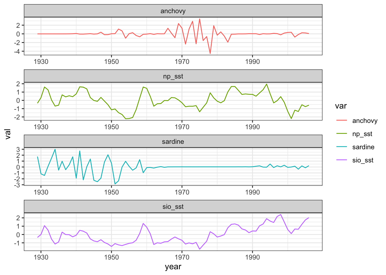
cmap <- CCM(dataFrame = sardine_anchovy_sst, E = 3, columns = "anchovy",
            target = "np_sst", libSizes = "10 70 10", sample = 100, showPlot = TRUE)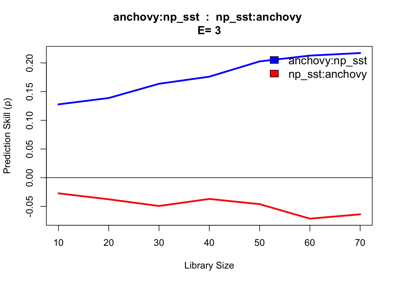
This CCM result anchovy::np_sst is interpreted as ‘sea surface temperature (np_sst) influences anchovy population,’ as you would expect since sea surface temperature can influence anchovy population size. The reverse direction (np_sst::anchovy) indicates no link, consistent with the fact that anchovy population does not influence sea surface temperature.
2.4 Example 3
From: https://github.com/SugiharaLab/rEDM
df = data.frame(yr = as.numeric(time(sunspot.year)),
                 sunspot_count = as.numeric(sunspot.year))

plot(df$yr, df$sunspot_count, type = "l",
     xlab = "year", ylab = "sunspots")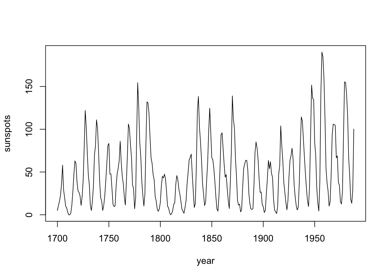
# translate = DO NOT RUN

df %>%
  ggplot(aes(x = yr, y = sunspot_count)) +
  geom_line() +
  labs(x = "year", y = "sunspots") +
  theme_bw()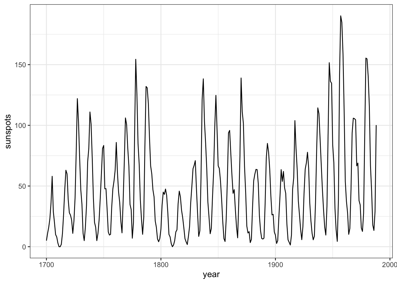
First, we use EmbedDimension() to determine the optimal embedding dimension, E:
E.opt = EmbedDimension( dataFrame = df,    # input data
                        lib     = "1 280", # portion of data to train
                        pred    = "1 280", # portion of data to predict
                        columns = "sunspot_count",
                        target  = "sunspot_count" )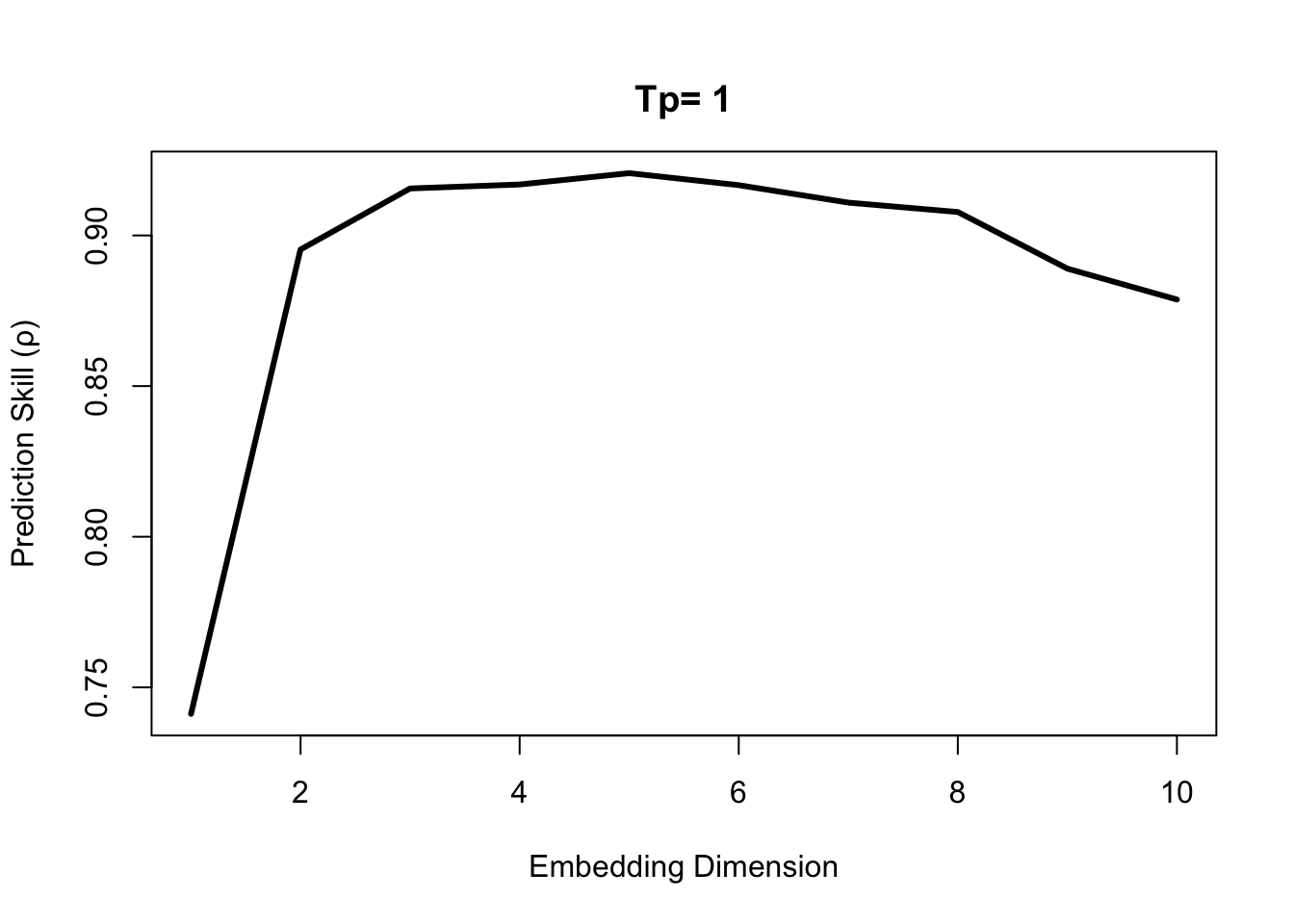
E.opt## E rho
## 1 1 0.7412040
## 2 2 0.8953335
## 3 3 0.9155983
## 4 4 0.9169173
## 5 5 0.9206748
## 6 6 0.9166970
## 7 7 0.9109041
## 8 8 0.9077828
## 9 9 0.8889942
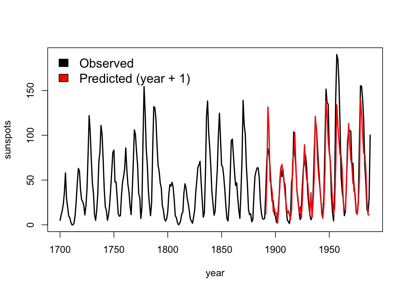
## 10 10 0.8787319Highest predictive skill is found between E = 3 and E = 6. Since we generally want a simpler model, if possible, we use E = 3 to forecast the last 1/3 of data based on training (attractor reconstruction) from the first 2/3.
simplex = Simplex( dataFrame = df,
                   lib     = "1   190", # portion of data to train
                   pred    = "191 287", # portion of data to predict
                   columns = "sunspot_count",
                   target  = "sunspot_count",
                   E       = 3 )
{
plot( df$yr, df$sunspot_count, type = "l", lwd = 2,
      xlab = "year", ylab = "sunspots")
lines( simplex$yr, simplex$Predictions, col = "red", lwd = 2)
legend( 'topleft', legend = c( "Observed", "Predicted (year + 1)" ),
        fill = c( 'black', 'red' ), bty = 'n', cex = 1.3 )
}
Extra: