Overview

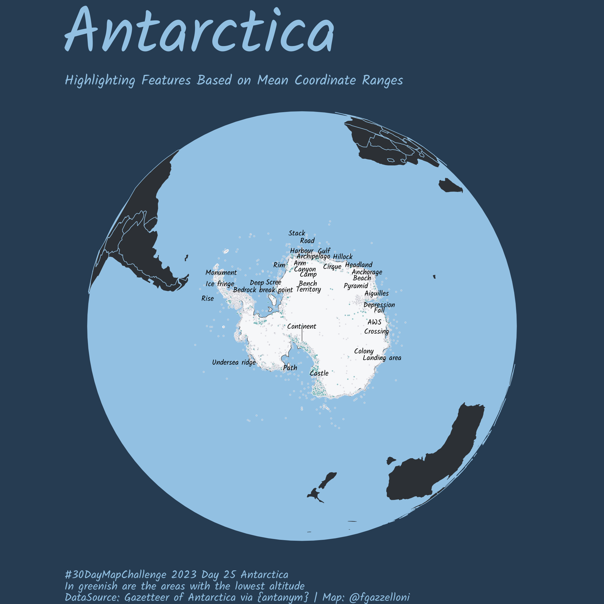
This is a Map of Antarctica made with the rOpenSci {antanym} package provided by

Composite Gazetteer of Antarctica, Scientific Committee on Antarctic Research. GCMD Metadata (http://gcmd.nasa.gov/records/SCAR_Gazetteer.html)

Load libraries

library(tidyverse)
library(sf)
library(elevatr)
library(showtext)
library(sysfonts)

Install and load the package also have a look at the documentation here: https://docs.ropensci.org/antanym/

# remotes::install_github("ropensci/antanym")
library(antanym)

Antarctic geographic place name information

The documentation recommend to use the cache and to select the names made available in “Poland” or “Germany” country languages.

g <- an_read(cache = "session")
# saveRDS(g,"data/g.rds")

g <- an_preferred(g, origin = c("Poland", "Germany"))
g%>%head

g%>%str

g%>%pull(altitude)%>%summary()

g%>%DataExplorer::profile_missing()

g_sf<- g%>%
  st_as_sf(coords=c("longitude","latitude"),crs=3031)

ggplot()+
  geom_sf(data=g_sf,aes(fill=altitude),
          shape=21,stroke=0.2,
          alpha=0.5,color="white")+
  scale_fill_viridis_c(direction = -1,begin = 0,end = 0.5)

Transform the projection following the example in the antanym-demo: - https://github.com/AustralianAntarcticDataCentre/antanym-demo

ortho<- "+proj=ortho +lat_0=-90 +lat_ts=-71 +lon_0=0 +k=1 +x_0=0 +y_0=0 +ellps=WGS84 +datum=WGS84 +units=m +no_defs"

Ocean

Set the buffer for drawing the ocean.

ocean <- st_point(x = c(0,0)) %>%
  st_buffer(dist = 6371000) %>% #6,371km ratios of the earth
  st_sfc(crs = ortho)

Load the World polygons with {tmap}:

library(tmap)
data("World")
# World

Transform the Antarctica locations points into a simple feature object, set the coordinate reference system (crs) to 4326 which is the standard point of view found in the world polygons.

g_sf<- g%>%
  st_as_sf(coords=c("longitude","latitude"),
           crs=4326)

g_text_sf <- g%>%
  group_by(feature_type_name)%>%
  reframe(longitude=mean(range(longitude)),
          latitude=mean(range(latitude)))%>%
  st_as_sf(coords=c("longitude","latitude"),
           crs=4326)

Make the Map

font_add_google(name = "Kalam", family = "Kalam")
showtext_auto()
showtext_opts(dpi = 320)

ocean

ggplot() + 
  geom_sf(data = ocean,
          linewidth=1,
          fill = "#92c0e2", 
          color = "#263c52")+
  geom_sf(data=World,fill="#2c3035",color="#92c0e2")+
  geom_sf(data=World%>%filter(name=="Antarctica"),fill="#f6f7f9")+
  geom_sf(data=g_sf,aes(fill=altitude),
          shape=21,stroke=0.2,
          size=0.5,
          alpha=0.5,color="white")+
  scale_fill_viridis_c(direction = -1,
                       begin = 0,end = 0.5,
                       na.value = "#bfc0ca")+
  geom_sf_text(data=g_text_sf,
               mapping=aes(label=feature_type_name),
               size=2,family="Kalam",
               check_overlap = T)+
  labs(title="Antarctica",
       subtitle="Highlighting Features Based on Mean Coordinate Ranges",
       caption="#30DayMapChallenge 2023 Day 25 Antarctica\nIn greenish are the areas with the lowest altitude\nDataSource: Gazetteer of Antarctica via {antanym} | Map: @fgazzelloni")+
  guides(fill="none")+
  coord_sf(crs=ortho)+
 theme_void(base_family = "Kalam")+
  theme(text=element_text(color="#92c0e2"),
        plot.title = element_text(size=50),
        plot.caption = element_text(hjust = 0))

ggsave("day25_antarctica.png",bg="#263c52")