Overview

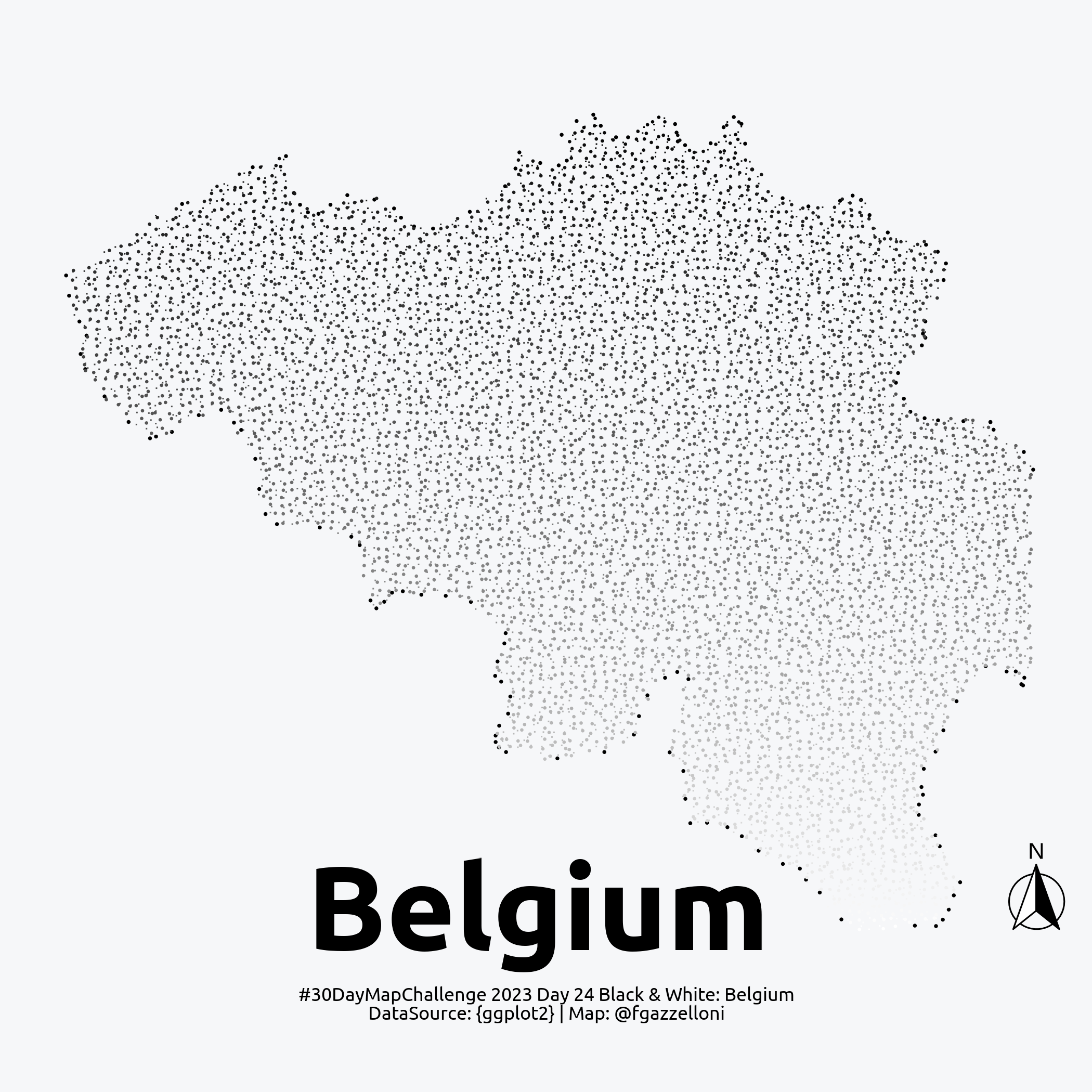
This Black & white Belgium Map is build creating a grid of points.

Load necessary libraries

library(tidyverse)
library(sf)
library(ggspatial)

library(showtext)
library(sysfonts)

library(maps)

library(DescTools)

font_add_google(name = "Ubuntu", family = "Ubuntu")
showtext_auto()
showtext_opts(dpi = 320)

Load the Belgium boundaries with map_data() function from the {ggplot2} package.

world <- map_data('world')
belgium<- world%>%
  filter(str_detect(region,"Belgium"))

Transform the Belgium dataset containing the longitude and latitude into a simple feature object with the st_as_sf() function from the {sf} package, and visualize the polygon. In this case is a POINT polygon.

bg_sf <- belgium%>%
  st_as_sf(coords = c("long","lat"))%>%
  st_make_valid()

ggplot(bg_sf)+
  geom_sf(color="grey40")+
  coord_sf()+
  theme_bw()

Let’s have a look at the same map witout transofrmation.

ggplot(belgium)+
  geom_polygon(aes(long,lat,group=group),fill="grey40")+
  coord_sf()+
  theme_bw()

In order to make a full grid of the Belgium polygon, the boundary box is extracted from the simple feature object with the st_bbox() function from the {sf} package.

bg_bbox <- bg_sf%>%
  st_bbox()

bg_bbox

Let’s first have a look at a simple perimeter grid with sf::st_make_grid() function, specifying the type of grid options, square = FALSE, and cellsize = .1.

grid <- bg_sf%>%
  sf::st_make_grid(square = FALSE,cellsize = .1)

Visualize the grid:

ggplot()+
  geom_sf(data=grid)+
  geom_sf(data=bg_sf)+
  coord_sf()+
  theme_bw()

min_lon <- bg_bbox[1]
max_lon <- bg_bbox[3]
min_lat <- bg_bbox[2]
max_lat <- bg_bbox[4]

And calculate the full grid of points:

bg_grid <- expand_grid(x = seq(from = min_lon, 
                               to = max_lon, length.out = 100),
                       y = seq(from = min_lat, 
                               to = max_lat, length.out = 100))

bg_coords <- belgium %>% 
  select(1:2) %>% 
  rename(x = long, y = lat)

In this case the application of the DescTools::PtInPoly() function builds points within the boundaries of a given polygon. The point in polygon, pip vector is created. The algorithm implements a sum of the angles made between the test point and each pair of points making up the polygon.

bg_grid_map <- data.frame(DescTools::PtInPoly(bg_grid, bg_coords)) %>% 
  filter(pip == 1) %>% 
  # group by latitude
  group_by(y) %>% 
  # set a new id vector for grouping points
  mutate(id = dplyr::cur_group_id()) %>%
  ungroup()

Make the map:

ggplot() +
  geom_jitter(data=belgium,
             aes(long,lat,group=group),size=0.2)+
  geom_jitter(data = bg_grid_map, 
          aes(x, y, group = id,color=y), 
          size=0.1,show.legend = F)+
  geom_jitter(data = bg_grid_map, 
            aes(x, y, group = id,color=y), 
            shape=".",show.legend = F) +
  scale_color_gradient(low = "white",high = "black") +
  scale_y_continuous(limits = c(49.5294835476, 51.4750237087)) +
  scale_x_continuous(limits = c(2.51357303225, 6.15665815596)) +
  coord_map(clip = "off") +
  annotate("text", y = 49.68, x = 4.3, 
           label = "Belgium", 
           family="Ubuntu",
           fontface = "bold", 
           size = 18, color = "#000000", vjust = "top") +
  ggspatial::annotation_north_arrow(location = "br", 
                         which_north = "true", 
                         pad_x = unit(0.0, "in"), 
                         pad_y = unit(0.2, "in"),
                         style = north_arrow_fancy_orienteering)+
   labs(caption = "#30DayMapChallenge 2023 Day 24 Black & White: Belgium\nDataSource: {ggplot2} | Map: @fgazzelloni")+
  ggthemes::theme_map() +
  theme(text = element_text(family="Ubuntu"),
        plot.caption = element_text( hjust = 0.5, 
                                     vjust=-0.1,
                                     size = 8),
        plot.caption.position = "plot")

ggsave("day_24_black&white.png",bg="#f6f7f9")