Overview

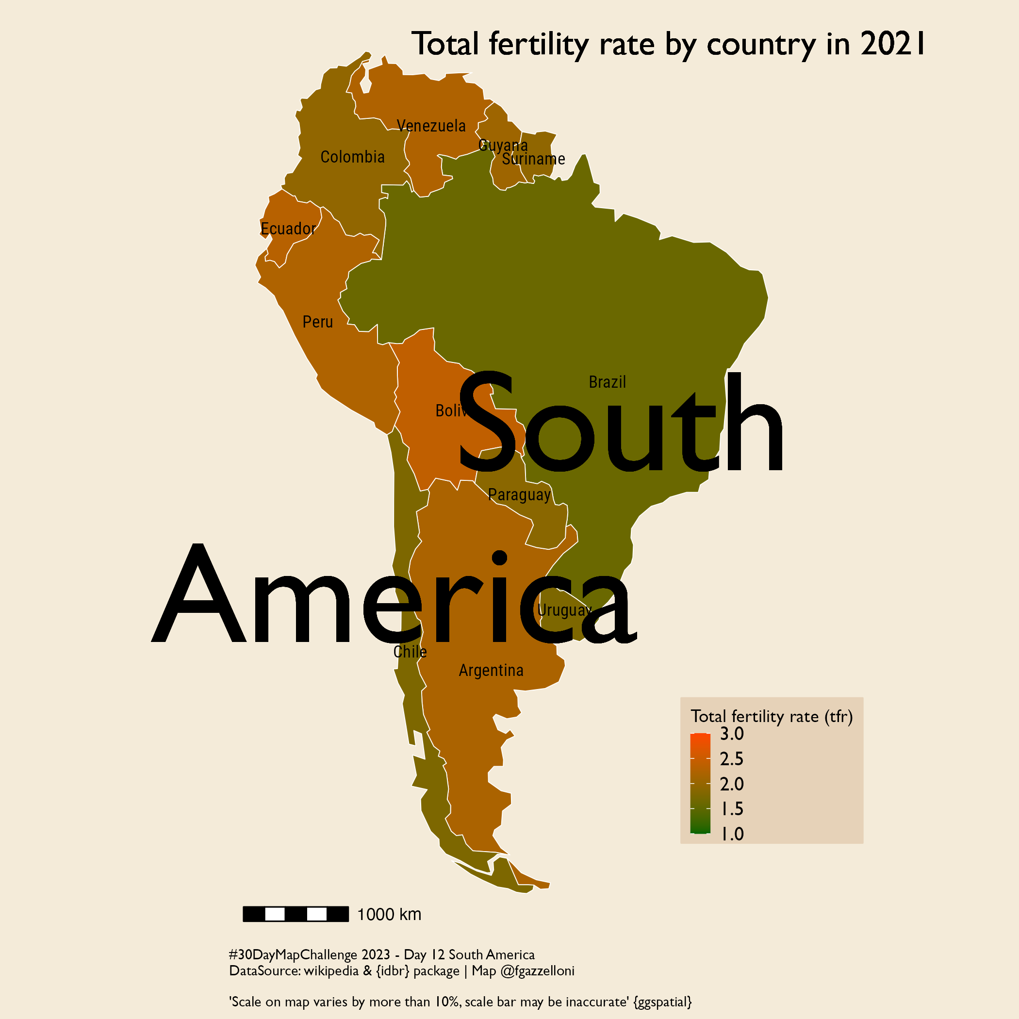
For this challenge I look back at day 8 Africa and the total fertility rate for replicating the steps for South America.

Datasource: Analyzing US Census Data: Methods, Maps, and Models in R, and the {idbr} package R Interface to the US Census Bureau International Data Base API.

Source: https://walker-data.com/census-r/working-with-census-data-outside-the-united-states.html

Census Data with {idbr}

Now you are all set to get ready downloading your favorite census data.

library(idbr)
library(tidyverse)

Get data for all countries

Here the tfr variable is selected as interested in the differences in total fertility rate in 2021 in South America.

data <- get_idb(
  country = "all",
  year = 2021,
  variables = "tfr",
  geometry = TRUE,
)

data %>% head()

Have a look at the global total fertility rate in 2021.

ggplot(data, aes(fill = code)) + 
  theme_bw() + 
  geom_sf() + 
  coord_sf(crs = 'ESRI:54030') + 
  scale_fill_viridis_d()+
  guides(fill=guide_legend(nrow = 10,title = ""))+
  theme(legend.key.size = unit(2,units = "pt"),
        legend.text = element_text(size=2),
        legend.position = "bottom")

Scrap the South America countries from Wikipedia:

https://en.wikipedia.org/wiki/South_America

library(rvest)

south_america_data <- read_html("https://en.wikipedia.org/wiki/South_America")

south_america_countries <- south_america_data %>%
  html_nodes("table") %>%
  .[[3]] %>%
  html_table(fill = TRUE)

south_america_countries %>% names()

south_america_countries <- south_america_countries%>%select('Country / Territory')%>%
  unlist()

Get the South America tfr data

sa <- get_idb(
  country = south_america_countries,
  year = 2021,
  variables = "tfr",
  geometry = TRUE,
)


sa %>% head()

Check the range of the tfr:

summary(sa$tfr)

Set a color range:

col.range<- c(1,3)

ggplot(sa, aes(fill = tfr)) + 
  geom_sf(color="white") + 
  geom_sf_text(aes(label=name),size=3,family="Roboto Condensed")+
  scale_fill_continuous(low = "#006400", 
                        high = "#FF4500",
                        limits=col.range)+
  ggtext::geom_richtext(x=0,y=0,
                        hjust = 2,
                        vjust=1.5,
                        label="South<br>America",
                        fill = NA, 
                        label.color = NA,
                        size=25,
                        family = "Gill Sans")+
    ggtext::geom_richtext(x=0,y=0,
                        hjust = 1.4,
                        vjust=-3,
                        label="Total fertility rate by country in 2021",
                        fill = NA, 
                        label.color = NA,
                        size=6,
                        family = "Gill Sans")+
  coord_sf(crs = 'ESRI:54030',clip = "off") + 
  labs(caption="#30DayMapChallenge 2023 - Day 12 South America\nDataSource: wikipedia & {idbr} package | Map @fgazzelloni\n\n'Scale on map varies by more than 10%, scale bar may be inaccurate' {ggspatial}",
       fill="Total fertility rate (tfr)")+
  ggthemes::theme_map()+
  theme(text=element_text(family = "Gill Sans"),
        plot.caption = element_text(hjust=0),
        legend.position = c(0.8,0.1),
        legend.key.size = unit(10,units = "pt"),
        legend.text = element_text(size=10),
        legend.background = element_rect(color="#E6D2B8",fill="#E6D2B8"))+
  ggspatial::annotation_scale()

Save it!

ggsave("day12_south-america.png",
       bg="#F4EBD9")