9  Word Embeddings

This session on word embeddings will conclude the script. Word embeddings are a fairly new technique that massively contributed to the progress the field of NLP has made over the last years. Their idea is basically that words can be embedded in a vector space in such a way that their real-life relationships are retained. This means for instance that words that co-appear in similar contexts are more similar – or have greater cosine similarity – than the ones that don’t. Also synonyms will be very similar.

In the following script, we will first use pre-trained (fasttext) embeddings to look a word relationships. Then, we will move on to train our own embeddings. This enables you to look at a typical application from the sociology of culture: determining how language is different across groups. In our particular case we will look at how certain gender stereotypes may be different in a sample of works of male and female authors downloaded using the gutenbergr package (and therefore quite old). I will leave the actual stereotype determination as an exercise for you though.

9.1 Pretrained embeddings

We will work with the fastText pretrained embeddings for English. They are downloaded once you click this link. Since they are huge, I will have to load them from my disc. I use data.table::fread() here.

needs(gutenbergr, gender, wordsalad, tidymodels, tidyverse, textrecipes, data.table, vip, ggrepel)
set.seed(123)

fasttext <- data.table::fread("/Users/felixlennert/Downloads/cc.en.300.vec", 
                              quote ="", 
                              skip = 1, 
                              data.table = F, 
                              nrows = 5e5)

9.2 Vector Algebra with pre-trained models

9.2.1 Word similarities

But let’s further investigate what’s going on under the hood of our fastText embeddings. We can use them to check out all things related to similarity of words: we can look for synonyms, investigate their relationships, and also visualize these quite conveniently by harnessing the power of dimensionality reduction.

What is powering these things is so-called cosine similarity: two vectors are the same if they “look into the same direction.” Cosine similarity is 0 if two vectors are orthogonal (90 degree angle), 1 if they are perfectly aligned, and -1 if they show in opposite directions.

Here, we will operate on the matrix as this is considerably faster than working with tibbles and dplyr function. For this, we first need to prepare the matrix.

fasttext_mat <- as.matrix(fasttext[, -1])
rownames(fasttext_mat) <- fasttext$V1

In a first task, we want to extract the best matches for a given word. Hence, we need a function that first calculates the cosine similarities of our term and then extracts the ones that actually have the highest cosine similarity.

## Function to get best matches
norms <- sqrt(rowSums(fasttext_mat^2)) # calculate length of vectors for normalization

best_match <- function(term, n = 5){
  x <- fasttext_mat[term, ]
  cosine <- (fasttext_mat %*% as.matrix(x)) / (norms * sqrt(sum(x^2))) # calculate cosine similarities between term in question and all the others
  best_n <- order(cosine, decreasing = T)[1:n] #extract highest n cosines
  tibble(
    word = rownames(fasttext_mat)[best_n], 
    cosine = cosine[best_n]
    )
}

Let’s check out some matches:

best_match("France", 10)

# A tibble: 10 × 2
   word       cosine
   <chr>       <dbl>
 1 France      1    
 2 France.The  0.742
 3 France-     0.704
 4 Paris       0.689
 5 Belgium     0.688
 6 Alsace      0.664
 7 Marseille   0.664
 8 France.     0.664
 9 Spain       0.664
10 Toulouse    0.658

best_match("Felix", 10)

# A tibble: 10 × 2
   word      cosine
   <chr>      <dbl>
 1 Felix      1    
 2 Norbert    0.605
 3 Félix      0.598
 4 Sebastian  0.598
 5 Matthias   0.595
 6 Fritz      0.594
 7 Gabriel    0.582
 8 Adrian     0.581
 9 Alex       0.579
10 Anton      0.576

best_match("Étienne", 10)

# A tibble: 10 × 2
   word          cosine
   <chr>          <dbl>
 1 Étienne        1    
 2 François       0.801
 3 Etienne        0.779
 4 Émile          0.737
 5 Jean-François  0.734
 6 Frédéric       0.724
 7 Jean-Pierre    0.720
 8 Benoît         0.718
 9 Jacques        0.718
10 Pierre         0.717

best_match("Julien", 10)

# A tibble: 10 × 2
   word      cosine
   <chr>      <dbl>
 1 Julien     1    
 2 Mathieu    0.729
 3 Maxime     0.721
 4 Philippe   0.712
 5 Stephane   0.706
 6 Jacques    0.706
 7 Etienne    0.697
 8 Sylvain    0.696
 9 Alexandre  0.695
10 Francois   0.695

We can also adapt the function to do some semantic algebra:

\[King - Man = ? - Woman\] \[King - Man + Woman = ?\]

semantic_algebra <- function(term_1, term_2, term_3, n = 5){
  x <- fasttext_mat[term_1, ] - fasttext_mat[term_2, ] + fasttext_mat[term_3, ]
  cosine <- (fasttext_mat %*% as.matrix(x)) / (norms * sqrt(sum(x^2))) # calculate cosine similarities between term in question and all the others
  best_n <- order(cosine, decreasing = T)[1:n] #extract highest n cosines
  tibble(
    word = rownames(fasttext_mat)[best_n], 
    cosine = cosine[best_n]
    )
}

semantic_algebra("king", "man", "woman")

# A tibble: 5 × 2
  word  cosine
  <chr>  <dbl>
1 king   0.729
2 queen  0.654
3 kings  0.541
4 Queen  0.507
5 royal  0.500

semantic_algebra("France", "Paris", "Rome")

# A tibble: 5 × 2
  word   cosine
  <chr>   <dbl>
1 Rome    0.862
2 Italy   0.710
3 Rome.   0.660
4 Latium  0.594
5 Sicily  0.592

9.2.2 Investigating biases

Quite in the same vein, we can also use vector algebra to investigate all different kinds of biases in language. The idea is to form certain dimensions or axes that relate to real-world spectra. Examples would be social class (“poor – rich”), gender (“male – female”), age (“young – old”).

investigate_bias <- function(axis_term_1, axis_term_2, term_in_question){
  x <- fasttext_mat[axis_term_2, ] - fasttext_mat[axis_term_1, ]
  tibble(
    axis_term_1 = axis_term_1,
    axis_term_2 = axis_term_2,
    term = term_in_question,
    cosine = lsa::cosine(x, fasttext_mat[term_in_question, ])
  )
}

investigate_bias("male", "female", "carpenter")

# A tibble: 1 × 4
  axis_term_1 axis_term_2 term      cosine[,1]
  <chr>       <chr>       <chr>          <dbl>
1 male        female      carpenter     -0.202

investigate_bias("male", "female", "secretary")

# A tibble: 1 × 4
  axis_term_1 axis_term_2 term      cosine[,1]
  <chr>       <chr>       <chr>          <dbl>
1 male        female      secretary   -0.00107

investigate_bias("male", "female", "stallion")

# A tibble: 1 × 4
  axis_term_1 axis_term_2 term     cosine[,1]
  <chr>       <chr>       <chr>         <dbl>
1 male        female      stallion     -0.275

investigate_bias("male", "female", "mare")

# A tibble: 1 × 4
  axis_term_1 axis_term_2 term  cosine[,1]
  <chr>       <chr>       <chr>      <dbl>
1 male        female      mare      -0.149

investigate_bias("male", "female", "Felix")

# A tibble: 1 × 4
  axis_term_1 axis_term_2 term  cosine[,1]
  <chr>       <chr>       <chr>      <dbl>
1 male        female      Felix     -0.157

investigate_bias("male", "female", "Felicia")

# A tibble: 1 × 4
  axis_term_1 axis_term_2 term    cosine[,1]
  <chr>       <chr>       <chr>        <dbl>
1 male        female      Felicia    -0.0671

9.2.3 Dimensionality Reduction

We can also reduce the dimensionality and put the terms into a two-dimensional representation (which is a bit easier to interpret for humans). To do this we perform a Principal Component Analysis and retain the first two components.

music_query <- c("Bach", "Mozart", "Haendel", "Verdi", "Bizet", "Poulenc", "Debussy", 
                 "Tupac", "Eminem", "Wu-Tang", 
                 "Coltrane", "Miles", "Armstrong", "Ellington", "Dolphy", "Hawkins")

name_query <- c("Julien", "Étienne", "Félix", 
                "Marie", "Anne", "Camille", 
                "Panagiotis", "Nikos", "Vassilis",
                "Maria", "Eugenia", "Myrto",
                "Khaled", "Karim", "Abdellatif",
                "Khalida", "Karima", "Aminata", 
                "Gunther", "Gunnar", "Anders", 
                "Greta", "Ursula", "Helga")

job_query <- c("economist", "sociologist", "psychologist", "anthropologist", 
               "historian", "geographer", "archeologist", "theologist")


music_pca <- prcomp(fasttext_mat[music_query, ]) |> 
  pluck("x") |> 
  as_tibble(rownames = NA) |> 
  rownames_to_column("name")

name_pca <- prcomp(fasttext_mat[name_query, ]) |> 
  pluck("x") |> 
  as_tibble(rownames = NA) |> 
  rownames_to_column("name")

job_pca <- prcomp(fasttext_mat[job_query, ]) |> 
  pluck("x") |> 
  as_tibble(rownames = NA) |> 
  rownames_to_column("name")

music_pca |> 
  ggplot() +
  geom_label_repel(aes(PC1, PC2, label = name))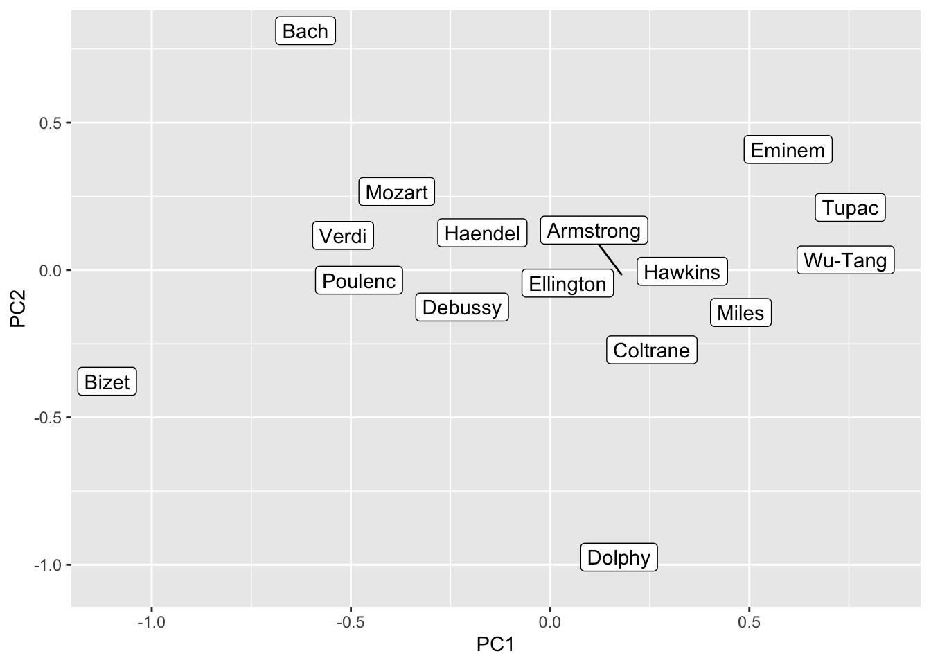

name_pca |> 
  ggplot() +
  geom_label_repel(aes(PC1, PC2, label = name))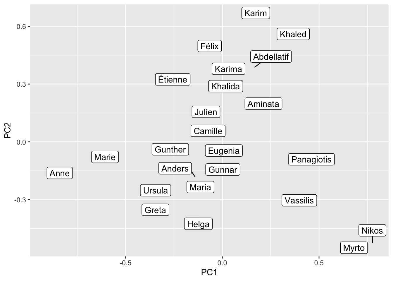

job_pca |> 
  ggplot() +
  geom_label_repel(aes(PC1, PC2, label = name)) +
  ylim(-0.5, 0.5) +
  xlim(-0.5, 0.5)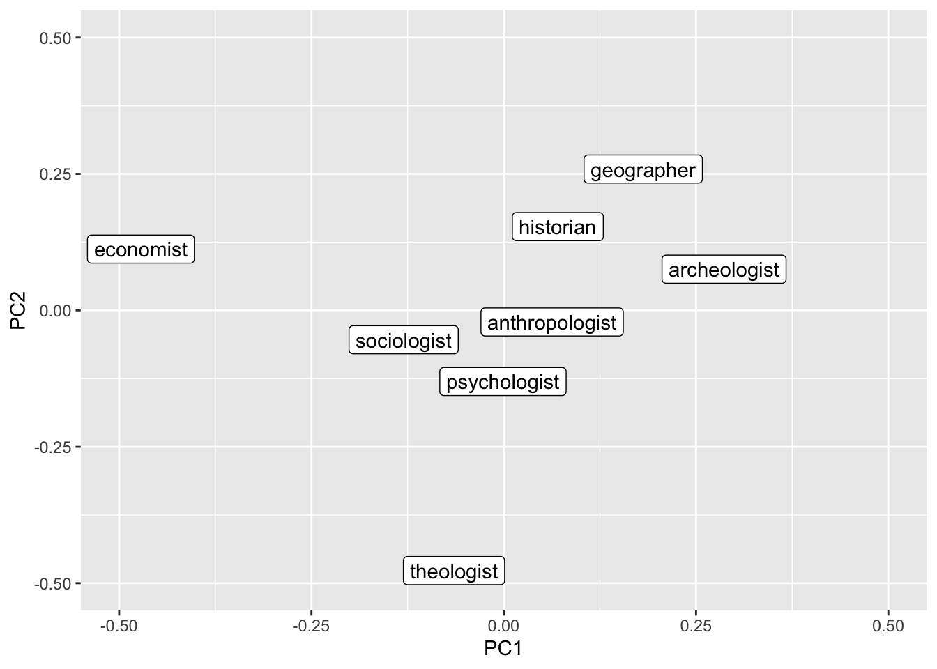

9.3 Train your own models

So far, this is all fun and games, but not so much suited for our research. If we want to do this, we need to be able to train the models ourselves. Then we can, for instance, systematically investigate the biases certain authors that bear certain traits (e.g., political leaning, born in the same century, same gender, skin color, etc.) have and how they compare to each other.

However, training these model requires a significant amount of text and a bit of computing power. Hence, in this example, we will look at books. This will give us some text. However, the books are all quite old – given that they come from the Gutenberg project (gutenbergr) and are therefore >70 years old. Also, we have little meta information on the authors. I will therefore use the gender package to infer their gender.

set.seed(123)

first_names <- gutenberg_metadata |> 
  filter(language == "en") |> 
  mutate(first_name = str_extract(author, "(?<=\\, )\\w+") |> 
           str_squish()) |> 
  replace_na(list(first_name = " ")) 

joined_names <- first_names |> 
  left_join(gender(first_names$first_name), by = c("first_name" = "name")) |> 
  distinct(gutenberg_id, .keep_all = TRUE) |> 
  drop_na(gender) |> 
  group_by(gender) |> 
  slice_sample(n = 100) |> 
  group_split()

male <- joined_names |> pluck(1) |> pull(gutenberg_id) |> gutenberg_download()
male_text <- male$text |> str_c(collapse = " ")
female <- joined_names |> pluck(2) |> pull(gutenberg_id) |> gutenberg_download()
female_text <- female$text |> str_c(collapse = " ")

#male_text |> write_rds("male_text.rds")
#female_text |> write_rds("female_text.rds")

Once we have acquired the text, we can train the models. Here, we will use the GloVe algorithm and lower dimensions. The wordsalad package provides us with an implementation.

male_emb <- wordsalad::glove(male_text |> str_remove_all("[:punct:]") |> str_to_lower())
male_emb_mat <- as.matrix(male_emb[, 2:11])
rownames(male_emb_mat) <- male_emb$tokens

female_emb <- wordsalad::glove(female_text |> str_remove_all("[:punct:]") |> str_to_lower())
female_emb_mat <- as.matrix(female_emb[, 2:11])
rownames(female_emb_mat) <- female_emb$tokens

Now we can use these matrices just as the pretrained matrix before and start to investigate different biases systematically. However, these biases are of course quite dependent on the choice of corpus. One way to mitigate this and to check the stability and robustness of the estimate would be a bootstrapping approach. Thereby, multiple models are trained with randomly sampled 95% of text units (e.g., sentences). Then, the bias estimates are calculated for each model and compared (Antoniak and Mimno 2018).

9.4 Further links

This is just a quick demonstration of what you can do with word embeddings. In case you want to use your embeddings as new features for your supervised machine learning classifier, look at ?textmodels::step_word_embeddings(). You may want to use pre-trained models for such tasks.

You can also train embeddings on multiple corpora and identify their different biases. You may want to have a look at (stoltz_cultural_2021?) before going down this road.

• See the word2vec vignette for more information
• The first of a series of blog posts on word embeddings
• An approachable lecture by Richard Socher, one of the founding fathers of GloVe

9.5 Exercises

1. Check out some analogies using the fastText embeddings.

2. Try to come up with your own axes. Play around and position words on them. Do your results always make sense? Inspiration can for instance be found in the works of Kozlowski, Taddy, and Evans (2019), or Garg et al. (2018).

3. Perform some queries on the PCA approach – do you find some good explanations for the patterns you see?

4. Compare the models we trained with the male- and female-authored corpora with regard to how “real-world gender-biased things” are biased in their texts. The functions from above will still work. Do you find differences?

female_emb_mat <- read_rds("https://www.dropbox.com/scl/fi/bk8iblukrzjih16ri2a16/female_glove_mat.rds?rlkey=q2udnazmyu2m024551nown3hh&dl=1")
male_emb_mat <- read_rds("https://www.dropbox.com/scl/fi/542fdz9wpy80yslduhxcz/male_glove_mat.rds?rlkey=gd1tkxzsxe1xaa59qzi3pqljj&dl=1")

Antoniak, Maria, and David Mimno. 2018. “Evaluating the Stability of Embedding-based Word Similarities.” Transactions of the Association for Computational Linguistics 6 (December): 107–19. https://doi.org/10.1162/tacl_a_00008.

Garg, Nikhil, Londa Schiebinger, Dan Jurafsky, and James Zou. 2018. “Word Embeddings Quantify 100 Years of Gender and Ethnic Stereotypes.” Proceedings of the National Academy of Sciences 115 (16): E3635–44. https://doi.org/10.1073/pnas.1720347115.

Kozlowski, Austin C., Matt Taddy, and James A. Evans. 2019. “The Geometry of Culture: Analyzing the Meanings of Class Through Word Embeddings.” American Sociological Review 84 (5): 905–49. https://doi.org/10.1177/0003122419877135.