6  Text Preprocessing and Featurization

After having learned about the basics of string manipulation, we are now turning to how you can turn your collection of documents, your corpus, into a representation that lends itself nicely to quantitative analyses of text. There are a couple of packages around which you can use for text mining, such as quanteda (Benoit et al. 2018), tm (Feinerer, Hornik, and Meyer 2008), and tidytext (Silge and Robinson 2016), the latter being probably the most recent addition to them. A larger overview of relevant packages can be found on this CRAN Task View.

As you could probably tell from its name, tidytext obeys the tidy data principles¹. “Every observation is a row” translates here to “every token has its own row” – “token” not necessarily relating to a singular term, but also so-called n-grams. In the following, we will demonstrate what text mining using tidy principles can look like in R. For this, we will first cover the preprocessing of text using tidy data principles. Thereafter, we will delve into more advanced preprocessing such as the lemmatization of words and part-of-speech (POS) tagging using spaCy (Honnibal and Montani 2017). Finally, different R packages are using different representations of text data. Depending on the task at hand, you will therefore have to be able to transform the data into the proper format. This will be covered in the final part.

6.1 Pre-processing with tidytext

The sotu package contains all of the so-called “State of the Union” addresses – the president gives them to the congress annually – since 1790.

needs(hcandersenr, SnowballC, sotu, spacyr, stopwords, tidyverse, tidytext)

sotu_raw <- sotu_meta |> 
  mutate(text = sotu_text) |> 
  distinct(text, .keep_all = TRUE)

sotu_raw |> glimpse()

Rows: 240
Columns: 7
$ X            <int> 1, 2, 3, 4, 5, 6, 7, 8, 9, 10, 11, 12, 13, 14, 15, 16, 17…
$ president    <chr> "George Washington", "George Washington", "George Washing…
$ year         <int> 1790, 1790, 1791, 1792, 1793, 1794, 1795, 1796, 1797, 179…
$ years_active <chr> "1789-1793", "1789-1793", "1789-1793", "1789-1793", "1793…
$ party        <chr> "Nonpartisan", "Nonpartisan", "Nonpartisan", "Nonpartisan…
$ sotu_type    <chr> "speech", "speech", "speech", "speech", "speech", "speech…
$ text         <chr> "Fellow-Citizens of the Senate and House of Representativ…

Now that the data are read in, I need to put them into the proper format and clean them. For this purpose, I take a look at the first entry of the tibble.

sotu_raw |> slice(1) |> pull(text) |> str_sub(1, 500)

[1] "Fellow-Citizens of the Senate and House of Representatives: \n\nI embrace with great satisfaction the opportunity which now presents itself of congratulating you on the present favorable prospects of our public affairs. The recent accession of the important state of North Carolina to the Constitution of the United States (of which official information has been received), the rising credit and respectability of our country, the general and increasing good will toward the government of the Union, an"

6.1.1 unnest_tokens()

I will focus on the 20th-century SOTUs. Here, the dplyr::between() function comes in handy.

sotu_20cent_raw <- sotu_raw |> 
  filter(between(year, 1900, 2000))

glimpse(sotu_20cent_raw)

Rows: 109
Columns: 7
$ X            <int> 112, 113, 114, 115, 116, 117, 118, 119, 120, 121, 122, 12…
$ president    <chr> "William McKinley", "Theodore Roosevelt", "Theodore Roose…
$ year         <int> 1900, 1901, 1902, 1903, 1904, 1905, 1906, 1907, 1908, 190…
$ years_active <chr> "1897-1901", "1901-1905", "1901-1905", "1901-1905", "1901…
$ party        <chr> "Republican", "Republican", "Republican", "Republican", "…
$ sotu_type    <chr> "written", "written", "written", "written", "written", "w…
$ text         <chr> "\n\n To the Senate and House of Representatives: \n\nAt …

In a first step, I bring the data into a form that facilitates manipulation: a tidy tibble. For this, I use tidytext’s unnest_tokens() function. It basically breaks the corpus up into tokens – the respective words. Let’s demonstrate that with a brief, intuitive example. `

toy_example <- tibble(
  text = "Look, this is a brief example for how tokenization works."
)

toy_example |> 
  unnest_tokens(output = token, 
                input = text)

# A tibble: 10 × 1
   token       
   <chr>       
 1 look        
 2 this        
 3 is          
 4 a           
 5 brief       
 6 example     
 7 for         
 8 how         
 9 tokenization
10 works       

Note that unnest_tokens() already reduces complexity for us by removing the comma and the full-stop and making everything lower-case.

sotu_20cent_tokenized <- sotu_20cent_raw |> 
  unnest_tokens(output = token, input = text)
glimpse(sotu_20cent_tokenized)

Rows: 911,321
Columns: 7
$ X            <int> 112, 112, 112, 112, 112, 112, 112, 112, 112, 112, 112, 11…
$ president    <chr> "William McKinley", "William McKinley", "William McKinley…
$ year         <int> 1900, 1900, 1900, 1900, 1900, 1900, 1900, 1900, 1900, 190…
$ years_active <chr> "1897-1901", "1897-1901", "1897-1901", "1897-1901", "1897…
$ party        <chr> "Republican", "Republican", "Republican", "Republican", "…
$ sotu_type    <chr> "written", "written", "written", "written", "written", "w…
$ token        <chr> "to", "the", "senate", "and", "house", "of", "representat…

The new tibble consists of 911321 rows. Please note that usually, you have to put some sort of id column into your original tibble before tokenizing it, e.g., by giving each case – representing a document, or chapter, or whatever – a separate id (e.g., using tibble::rowid_to_column()). This does not apply here, because my original tibble came with a bunch of metadata (president, year, party) which serve as sufficient identifiers.

6.1.2 Removal of unnecessary content

The next step is to remove stop words – they are not necessary for the analyses I want to perform. The stopwords package has a nice list for English.

stopwords_vec <- stopwords(language = "en")
stopwords(language = "de") # the german equivalent

  [1] "aber"      "alle"      "allem"     "allen"     "aller"     "alles"    
  [7] "als"       "also"      "am"        "an"        "ander"     "andere"   
 [13] "anderem"   "anderen"   "anderer"   "anderes"   "anderm"    "andern"   
 [19] "anderr"    "anders"    "auch"      "auf"       "aus"       "bei"      
 [25] "bin"       "bis"       "bist"      "da"        "damit"     "dann"     
 [31] "der"       "den"       "des"       "dem"       "die"       "das"      
 [37] "daß"       "derselbe"  "derselben" "denselben" "desselben" "demselben"
 [43] "dieselbe"  "dieselben" "dasselbe"  "dazu"      "dein"      "deine"    
 [49] "deinem"    "deinen"    "deiner"    "deines"    "denn"      "derer"    
 [55] "dessen"    "dich"      "dir"       "du"        "dies"      "diese"    
 [61] "diesem"    "diesen"    "dieser"    "dieses"    "doch"      "dort"     
 [67] "durch"     "ein"       "eine"      "einem"     "einen"     "einer"    
 [73] "eines"     "einig"     "einige"    "einigem"   "einigen"   "einiger"  
 [79] "einiges"   "einmal"    "er"        "ihn"       "ihm"       "es"       
 [85] "etwas"     "euer"      "eure"      "eurem"     "euren"     "eurer"    
 [91] "eures"     "für"       "gegen"     "gewesen"   "hab"       "habe"     
 [97] "haben"     "hat"       "hatte"     "hatten"    "hier"      "hin"      
[103] "hinter"    "ich"       "mich"      "mir"       "ihr"       "ihre"     
[109] "ihrem"     "ihren"     "ihrer"     "ihres"     "euch"      "im"       
[115] "in"        "indem"     "ins"       "ist"       "jede"      "jedem"    
[121] "jeden"     "jeder"     "jedes"     "jene"      "jenem"     "jenen"    
[127] "jener"     "jenes"     "jetzt"     "kann"      "kein"      "keine"    
[133] "keinem"    "keinen"    "keiner"    "keines"    "können"    "könnte"   
[139] "machen"    "man"       "manche"    "manchem"   "manchen"   "mancher"  
[145] "manches"   "mein"      "meine"     "meinem"    "meinen"    "meiner"   
[151] "meines"    "mit"       "muss"      "musste"    "nach"      "nicht"    
[157] "nichts"    "noch"      "nun"       "nur"       "ob"        "oder"     
[163] "ohne"      "sehr"      "sein"      "seine"     "seinem"    "seinen"   
[169] "seiner"    "seines"    "selbst"    "sich"      "sie"       "ihnen"    
[175] "sind"      "so"        "solche"    "solchem"   "solchen"   "solcher"  
[181] "solches"   "soll"      "sollte"    "sondern"   "sonst"     "über"     
[187] "um"        "und"       "uns"       "unse"      "unsem"     "unsen"    
[193] "unser"     "unses"     "unter"     "viel"      "vom"       "von"      
[199] "vor"       "während"   "war"       "waren"     "warst"     "was"      
[205] "weg"       "weil"      "weiter"    "welche"    "welchem"   "welchen"  
[211] "welcher"   "welches"   "wenn"      "werde"     "werden"    "wie"      
[217] "wieder"    "will"      "wir"       "wird"      "wirst"     "wo"       
[223] "wollen"    "wollte"    "würde"     "würden"    "zu"        "zum"      
[229] "zur"       "zwar"      "zwischen" 

#stopwords_getlanguages(source = "snowball") # find the languages that are available
#stopwords_getsources() # find the dictionaries that are available

Removing the stop words now is straight-forward:

sotu_20cent_tokenized_nostopwords <- sotu_20cent_tokenized |> 
  filter(!token %in% stopwords_vec)

Another thing I forgot to remove are digits. They do not matter for the analyses either:

sotu_20cent_tokenized_nostopwords_nonumbers <- sotu_20cent_tokenized_nostopwords |> 
  filter(!str_detect(token, "[:digit:]"))

The corpus now contains 19263 different tokens, the so-called “vocabulary.” 1848 tokens were removed from the vocuabulary. This translates to a signifiant reduction in corpus size though, the new tibble only consists of 464271 rows, basically a 50 percent reduction.

6.1.3 Stemming

To decrease the complexity of the vocabulary even further, we can reduce the tokens to their stem using the SnowballC package and its function wordStem():

sotu_20cent_tokenized_nostopwords_nonumbers_stemmed <- sotu_20cent_tokenized_nostopwords_nonumbers |> 
  mutate(token_stemmed = wordStem(token, language = "en"))

#SnowballC::getStemLanguages() # if you want to know the abbreviations for other languages as well

Maybe I should also remove insignificant words, i.e., ones that appear less than 0.05 percent of the time.

n_rows <- nrow(sotu_20cent_tokenized_nostopwords_nonumbers_stemmed)
sotu_20cent_tokenized_nostopwords_nonumbers_stemmed |> 
  group_by(token_stemmed) |> 
  filter(n() > n_rows/2000)

# A tibble: 285,203 × 8
# Groups:   token_stemmed [490]
       X president         year years_active party sotu_type token token_stemmed
   <int> <chr>            <int> <chr>        <chr> <chr>     <chr> <chr>        
 1   112 William McKinley  1900 1897-1901    Repu… written   sena… senat        
 2   112 William McKinley  1900 1897-1901    Repu… written   house hous         
 3   112 William McKinley  1900 1897-1901    Repu… written   repr… repres       
 4   112 William McKinley  1900 1897-1901    Repu… written   old   old          
 5   112 William McKinley  1900 1897-1901    Repu… written   inco… incom        
 6   112 William McKinley  1900 1897-1901    Repu… written   new   new          
 7   112 William McKinley  1900 1897-1901    Repu… written   cent… centuri      
 8   112 William McKinley  1900 1897-1901    Repu… written   begin begin        
 9   112 William McKinley  1900 1897-1901    Repu… written   last  last         
10   112 William McKinley  1900 1897-1901    Repu… written   sess… session      
# ℹ 285,193 more rows

These steps have brought down the vocabulary from 19263 to 10971.

6.1.4 In a nutshell

Well, all those things could also be summarized in one nice cleaning pipeline:

sotu_20cent_clean <- sotu_raw |> 
  filter(between(year, 1900, 2000)) |> 
  unnest_tokens(output = token, input = text) |> 
  anti_join(get_stopwords(), by = c("token" = "word")) |> 
  filter(!str_detect(token, "[0-9]")) |> 
  mutate(token = wordStem(token, language = "en")) |> 
  group_by(token) |> 
  filter(n() > n_rows/2000)

Now I have created a nice tibble containing the SOTU addresses of the 20th century in a tidy format. This is a great point of departure for subsequent analyses.

6.1.5 Exercises

1. Download Twitter timeline data (timelines <- read_csv("https://www.dropbox.com/s/dpu5m3xqz4u4nv7/tweets_house_rep_party.csv?dl=1") |> filter(!is.na(party)). Let’s look at abortion-related tweets and how the language may differ between parties. Filter relevant tweets using a vector of keywords and a regular expression (hint: filter(str_detect(text, str_c(keywords, collapse = "|")))). Preprocess the Tweets as follows:

1. Unnest the tokens.
2. Remove stop words.
3. Perform stemming.

needs(tidyverse, tidytext, stopwords, SnowballC)

timelines <- read_csv("https://www.dropbox.com/s/dpu5m3xqz4u4nv7/tweets_house_rep_party.csv?dl=1") |> 
  filter(!is.na(party))

keywords <- c("abortion", "prolife", " roe ", " wade ", "roevswade", "baby", "fetus", "womb", "prochoice", "leak")

preprocessed <- timelines |> 
  rowid_to_column("doc_id") |> 
  filter(str_detect(text, str_c(keywords, collapse = "|"))) |> 
  unnest_tokens(word, text) |> 
  anti_join(get_stopwords()) |> 
  mutate(stemmed = wordStem(word))

6.2 Lemmatization, Named Entity Recognition, POS-tagging, and Dependency Parsing with spaCyR

Advanced operations to the end of extracting information and annotating text (and more!) can be done with spaCyr (Benoit and Matsuo 2020). spaCyr is an R wrapper around the spaCy Python package and, therefore, a bit tricky to install at first. You can find instructions here.

The functionalities spaCyr offers you are the following²:

• parsing texts into tokens or sentences;
• lemmatizing tokens;
• parsing dependencies (to identify the grammatical structure of the sentence); and
• identifying, extracting, or consolidating token sequences that form named entities or noun phrases.

In brief, preprocessing with spaCyr is computationally more expensive than using, for instance, tidytext, but it will give you more accurate lemmatization instead of “stupid,” rule-based stemming.. Also, it allows you to break up documents into smaller entities, sentences, which might be more suitable, e.g., as input for classifiers (since sentences tend to be about one topic, they allow for more fine-grained analyses). Part-of-speech (POS) tagging basically provides you with the functions of the different terms within the sentence. This might prove useful for tasks such as sentiment analysis. The final task spaCyr can help you with is Named Entity Recognition (NER) which can be used for tasks such as sampling relevant documents.

6.2.1 Initializing spaCy

Before using spaCyr, it needs to be initialized. What happens during this process is that R basically opens a connection to Python so that it can then run the spaCyr functions in Python’s spaCy. Once you have set up everything properly (see instructions), you can initialize it using spacy_initialize(model). Different language models can be specified and an overview can be found here. Note that a process of spaCy is started when you spacy_initialize() and continues running in the background. Hence, once you don’t need it anymore, or want to load a different model, you should spacy_finalize().

needs(spacyr)
spacy_initialize(model = "en_core_web_sm")

Found 'spacy_condaenv'. spacyr will use this environment

successfully initialized (spaCy Version: 3.3.0, language model: en_core_web_sm)

(python options: type = "condaenv", value = "spacy_condaenv")

# to download new model -- here: French
#spacy_finalize()
#spacy_download_langmodel(model = "fr_core_news_sm")
#spacy_initialize(model = "fr_core_news_sm") #check that it has worked

spacy_finalize()
#spacy_initialize(model = "de_core_web_sm") # for German

6.2.2 spacy_parse()

spaCyr’s workhorse function is spacy_parse(). It takes a character vector or TIF-compliant data frame. The latter is basically a tibble containing at least two columns, one named doc_id with unique document ids and one named text, containing the respective documents.

tif_toy_example <- tibble(
  doc_id = "doc1",
  text = "Look, this is a brief example for how tokenization works. This second sentence allows me to demonstrate another functionality of spaCy."
)

toy_example_vec <- tif_toy_example$text

spacy_parse(tif_toy_example)

Python space is already attached.  If you want to switch to a different Python, please restart R.

successfully initialized (spaCy Version: 3.3.0, language model: en_core_web_sm)

(python options: type = "condaenv", value = "spacy_condaenv")

   doc_id sentence_id token_id         token         lemma   pos    entity
1    doc1           1        1          Look          look  VERB          
2    doc1           1        2             ,             , PUNCT          
3    doc1           1        3          this          this  PRON          
4    doc1           1        4            is            be   AUX          
5    doc1           1        5             a             a   DET          
6    doc1           1        6         brief         brief   ADJ          
7    doc1           1        7       example       example  NOUN          
8    doc1           1        8           for           for   ADP          
9    doc1           1        9           how           how SCONJ          
10   doc1           1       10  tokenization  tokenization  NOUN          
11   doc1           1       11         works          work  VERB          
12   doc1           1       12             .             . PUNCT          
13   doc1           2        1          This          this   DET          
14   doc1           2        2        second        second   ADJ ORDINAL_B
15   doc1           2        3      sentence      sentence  NOUN          
16   doc1           2        4        allows         allow  VERB          
17   doc1           2        5            me             I  PRON          
18   doc1           2        6            to            to  PART          
19   doc1           2        7   demonstrate   demonstrate  VERB          
20   doc1           2        8       another       another   DET          
21   doc1           2        9 functionality functionality  NOUN          
22   doc1           2       10            of            of   ADP          
23   doc1           2       11         spaCy         spaCy PROPN          
24   doc1           2       12             .             . PUNCT          

The output of spacy_parse() and the sotu-speeches looks as follows:

sotu_speeches_tif <- sotu_meta |> 
  mutate(text = sotu_text) |> 
  distinct(text, .keep_all = TRUE) |> 
  filter(between(year, 1990, 2000)) |> 
  group_by(year) |> 
  summarize(text = str_c(text, collapse = " ")) |> 
  select(doc_id = year, text)

glimpse(sotu_speeches_tif)

Rows: 11
Columns: 2
$ doc_id <int> 1990, 1991, 1992, 1993, 1994, 1995, 1996, 1997, 1998, 1999, 2000
$ text   <chr> "\n\nMr. President, Mr. Speaker, Members of the United States C…

sotu_parsed <- spacy_parse(sotu_speeches_tif,
                           pos = TRUE,
                           tag = TRUE,
                           lemma = TRUE,
                           entity = TRUE,
                           dependency = TRUE,
                           nounphrase = TRUE,
                           multithread = TRUE)

# if you haven't installed spacy yet, uncomment and run the following line
#sotu_parsed <- read_rds("https://github.com/fellennert/sicss-paris-2023/raw/main/code/sotu_parsed.rds")

Note that this is already fairly similar to the output of tidytext’s unnest_tokens() function. The advantages are that the lemmas are more accurate, that we have a new sub-entity – sentences –, and that there is now more information on the type and meanings of the words.

6.2.3 POS tags, NER, and nounphrases

The abbreviations in the pos column follow the format of Universal POS tags. Entities can be extracted by passing the parsed object on to entity_extract().

entity_extract(sotu_parsed, type = "all") |> glimpse()

Rows: 4,078
Columns: 4
$ doc_id      <chr> "1990", "1990", "1990", "1990", "1990", "1990", "1990", "1…
$ sentence_id <int> 1, 1, 1, 1, 3, 4, 4, 6, 6, 6, 6, 7, 9, 10, 10, 11, 11, 12,…
$ entity      <chr> "Speaker", "the_United_States", "Senate", "House", "the_co…
$ entity_type <chr> "PERSON", "ORG", "ORG", "ORG", "DATE", "NORP", "GPE", "ORG…

The following entities are recognized (overview taken from this article):

• PERSON: People, including fictional.
• NORP: Nationalities or religious or political groups.
• FAC: Buildings, airports, highways, bridges, etc.
• ORG: Companies, agencies, institutions, etc.
• GPE: Countries, cities, states.
• LOC: Non-GPE locations, mountain ranges, bodies of water.
• PRODUCT: Objects, vehicles, foods, etc. (Not services.)
• EVENT: Named hurricanes, battles, wars, sports events, etc.
• WORK_OF_ART: Titles of books, songs, etc.
• LAW: Named documents made into laws.
• LANGUAGE: Any named language.
• DATE: Absolute or relative dates or periods.
• TIME: Times smaller than a day.
• PERCENT: Percentage, including “%”.
• MONEY: Monetary values, including unit.
• QUANTITY: Measurements, as of weight or distance.
• ORDINAL: “first,” “second,” etc.
• CARDINAL: Numerals that do not fall under another type.

To properly represent entities in our corpus, you can use entity_consolidate(). This collapses words that belong to the same entity into single tokens (e.g., “the” “white” “house” becomes “the_white_house”).

entity_consolidate(sotu_parsed) |> glimpse()

Note: removing head_token_id, dep_rel for named entities

Rows: 81,824
Columns: 8
$ doc_id      <chr> "1990", "1990", "1990", "1990", "1990", "1990", "1990", "1…
$ sentence_id <int> 1, 1, 1, 1, 1, 1, 1, 1, 1, 1, 1, 1, 1, 1, 1, 1, 1, 1, 1, 1…
$ token_id    <dbl> 1, 2, 3, 4, 5, 6, 7, 8, 9, 10, 11, 12, 13, 14, 15, 16, 17,…
$ token       <chr> "\n\n", "Mr.", "President", ",", "Mr.", "Speaker", ",", "M…
$ lemma       <chr> "\n\n", "Mr.", "President", ",", "Mr.", "Speaker", ",", "M…
$ pos         <chr> "SPACE", "PROPN", "PROPN", "PUNCT", "PROPN", "ENTITY", "PU…
$ tag         <chr> "_SP", "NNP", "NNP", ",", "NNP", "ENTITY", ",", "NNP", "IN…
$ entity_type <chr> "", "", "", "", "", "PERSON", "", "", "", "ORG", "", "", "…

If you want to extract only nouns, you can simply filter them.

sotu_parsed |> 
  entity_consolidate() |> 
  filter(pos == "NOUN") |> 
  glimpse()

Note: removing head_token_id, dep_rel for named entities

Rows: 14,220
Columns: 8
$ doc_id      <chr> "1990", "1990", "1990", "1990", "1990", "1990", "1990", "1…
$ sentence_id <int> 2, 2, 3, 3, 3, 3, 3, 4, 4, 4, 4, 4, 5, 5, 6, 6, 6, 6, 6, 6…
$ token_id    <dbl> 10, 17, 2, 10, 20, 29, 32, 12, 15, 22, 25, 31, 5, 7, 13, 1…
$ token       <chr> "privilege", "state", "Tonight", "state", "initiative", "l…
$ lemma       <chr> "privilege", "state", "tonight", "state", "initiative", "l…
$ pos         <chr> "NOUN", "NOUN", "NOUN", "NOUN", "NOUN", "NOUN", "NOUN", "N…
$ tag         <chr> "NN", "NN", "NN", "NN", "NN", "NN", "NN", "NNS", "NN", "NN…
$ entity_type <chr> "", "", "", "", "", "", "", "", "", "", "", "", "", "", ""…

However, a better way is to extract the “complete” noun phrases:

nounphrase_extract(sotu_parsed) |> glimpse()

Rows: 21,548
Columns: 3
$ doc_id      <chr> "1990", "1990", "1990", "1990", "1990", "1990", "1990", "1…
$ sentence_id <int> 1, 1, 1, 1, 1, 1, 1, 1, 1, 2, 2, 2, 2, 2, 2, 3, 3, 3, 3, 3…
$ nounphrase  <chr> "Mr._President", "Mr._Speaker", "Members", "the_United_Sta…

Usually, entities and noun phrases can give you a good idea of what texts are about. Therefore, you might want to only extract them without parsing the entire text.

spacy_extract_entity(sotu_speeches_tif |> slice(1:3)) |> glimpse()

Rows: 675
Columns: 5
$ doc_id   <chr> "1990", "1990", "1990", "1990", "1990", "1990", "1990", "1990…
$ text     <chr> "Speaker", "the United States", "Senate", "House", "the comin…
$ ent_type <chr> "PERSON", "ORG", "ORG", "ORG", "DATE", "NORP", "GPE", "ORG", …
$ start_id <dbl> 6, 10, 24, 32, 78, 100, 129, 158, 174, 180, 197, 206, 243, 28…
$ length   <int> 1, 3, 1, 1, 3, 1, 1, 1, 1, 2, 1, 3, 2, 4, 1, 3, 1, 1, 1, 1, 1…

spacy_extract_nounphrases(sotu_speeches_tif |> slice(1:3)) |> glimpse()

Rows: 3,873
Columns: 6
$ doc_id    <chr> "1990", "1990", "1990", "1990", "1990", "1990", "1990", "199…
$ text      <chr> "Mr. President", "Mr. Speaker", "Members", "the United State…
$ root_text <chr> "President", "Speaker", "Members", "Congress", "I", "Preside…
$ start_id  <dbl> 2, 5, 8, 10, 16, 19, 23, 26, 30, 38, 40, 42, 47, 49, 52, 57,…
$ root_id   <dbl> 3, 6, 8, 13, 16, 21, 24, 28, 32, 38, 40, 43, 47, 50, 53, 57,…
$ length    <int> 2, 2, 1, 4, 1, 3, 2, 3, 3, 1, 1, 2, 1, 2, 2, 1, 2, 2, 3, 1, …

6.2.4 Exercises

2. Perform the same steps as in exercise 1 but using spacyr. What works better, lemmatization or stemming?

needs(spacyr)
spacy_initialize(model = "en_core_web_sm")

timelines_meta <- timelines |> 
  filter(str_detect(text, str_c(keywords, collapse = "|"))) |> 
  rowid_to_column("doc_id") |> 
  select(-text)

timelines_spacy <- timelines |> 
  filter(str_detect(text, str_c(keywords, collapse = "|"))) |> 
  select(text) |> 
  rowid_to_column("doc_id") |> 
  spacy_parse(entity = FALSE) |> 
  anti_join(get_stopwords(), by = c("token" = "word"))

6.3 Converting between formats

While the tidytext format lends itself nicely to “basic” operations and visualizations, you will have to use different representations of text data for other applications such as topic models or word embeddings. On the other hand, you might want to harness, for instance, the ggplot2 package for visualization. In this case, you will need to project the data into a tidy format. The former operations are performed using multiple cast_.*() functions, the latter using the tidy() function from the broom package whose purpose is to bring data from foreign structures to tidy representations.

In the following, I will briefly explain common representations and the packages that use them. Thereby, I draw heavily on the chapter in Tidy Text Mining with R that is dedicated to the topic.

6.3.1 Document-term matrix

A document-term matrix contains rows that represent a document and columns that represent terms. The values usually correspond to how often the term appears in the respective document.

In R, a common implementation of DTMs is the DocumentTermMatrix class in the tm package. The topicmodels package which we will use for performing LDA comes with a collection of example data.

library(topicmodels)
data("AssociatedPress")

class(AssociatedPress)

[1] "DocumentTermMatrix"    "simple_triplet_matrix"

AssociatedPress

<<DocumentTermMatrix (documents: 2246, terms: 10473)>>
Non-/sparse entries: 302031/23220327
Sparsity           : 99%
Maximal term length: 18
Weighting          : term frequency (tf)

This data set contains 2246 Associated Press articles which consist of 10,473 different terms. Moreover, the matrix is 99% sparse, meaning that 99% of word-document pairs are zero. The weighting is by term frequency, hence the values correspond to the number of appearances a word has in an article.

AssociatedPress |> 
  head(2) |> 
  as.matrix() %>%
  .[, 1:10]

      Terms
Docs   aaron abandon abandoned abandoning abbott abboud abc abcs abctvs abdomen
  [1,]     0       0         0          0      0      0   0    0      0       0
  [2,]     0       0         0          0      0      0   0    0      0       0

Bringing these data into a tidy format is performed as follows:

associated_press_tidy <- tidy(AssociatedPress)

glimpse(associated_press_tidy)

Rows: 302,031
Columns: 3
$ document <int> 1, 1, 1, 1, 1, 1, 1, 1, 1, 1, 1, 1, 1, 1, 1, 1, 1, 1, 1, 1, 1…
$ term     <chr> "adding", "adult", "ago", "alcohol", "allegedly", "allen", "a…
$ count    <dbl> 1, 2, 1, 1, 1, 1, 2, 1, 1, 1, 2, 1, 1, 2, 1, 1, 1, 1, 4, 4, 1…

Transforming the data set into a DTM, the opposite operation, is achieved using cast_dtm(data, document, term, value):

associated_press_dfm <- associated_press_tidy |> 
  cast_dtm(document, term, count)

associated_press_dfm |> 
  head(2) |> 
  as.matrix() %>%
  .[, 1:10]

    Terms
Docs adding adult ago alcohol allegedly allen apparently appeared arrested
   1      1     2   1       1         1     1          2        1        1
   2      0     0   0       0         0     0          0        1        0
    Terms
Docs assault
   1       1
   2       0

6.3.2 Document-feature matrix

The so-called document-feature matrix is the data format used in the quanteda package. It is basically a document-term matrix, but the authors of the quanteda package chose the term feature over term to be more accurate:

“We call them ‘features’ rather than terms, because features are more general than terms: they can be defined as raw terms, stemmed terms, the parts of speech of terms, terms after stopwords have been removed, or a dictionary class to which a term belongs. Features can be entirely general, such as ngrams or syntactic dependencies, and we leave this open-ended.”

data("data_corpus_inaugural", package = "quanteda")
inaug_dfm <- data_corpus_inaugural |>
  quanteda::tokens() |>
  quanteda::dfm(verbose = FALSE)

inaug_dfm

Document-feature matrix of: 59 documents, 9,441 features (91.84% sparse) and 4 docvars.
                 features
docs              fellow-citizens  of the senate and house representatives :
  1789-Washington               1  71 116      1  48     2               2 1
  1793-Washington               0  11  13      0   2     0               0 1
  1797-Adams                    3 140 163      1 130     0               2 0
  1801-Jefferson                2 104 130      0  81     0               0 1
  1805-Jefferson                0 101 143      0  93     0               0 0
  1809-Madison                  1  69 104      0  43     0               0 0
                 features
docs              among vicissitudes
  1789-Washington     1            1
  1793-Washington     0            0
  1797-Adams          4            0
  1801-Jefferson      1            0
  1805-Jefferson      7            0
  1809-Madison        0            0
[ reached max_ndoc ... 53 more documents, reached max_nfeat ... 9,431 more features ]

This, again, can just be tidy()ed.

inaug_tidy <- tidy(inaug_dfm)

glimpse(inaug_tidy)

Rows: 45,454
Columns: 3
$ document <chr> "1789-Washington", "1797-Adams", "1801-Jefferson", "1809-Madi…
$ term     <chr> "fellow-citizens", "fellow-citizens", "fellow-citizens", "fel…
$ count    <dbl> 1, 3, 2, 1, 1, 5, 1, 11, 1, 1, 2, 1, 1, 2, 1, 1, 1, 2, 1, 71,…

Of course, the resulting tibble can now be cast back into the DFM format using cast_dfm(data, document, term, value). Here, the value corresponds to the number of appearances of the term in the respective document.

inaug_tidy |> 
  cast_dfm(document, term, count)

Document-feature matrix of: 59 documents, 9,441 features (91.84% sparse) and 0 docvars.
                 features
docs              fellow-citizens  of the senate and house representatives :
  1789-Washington               1  71 116      1  48     2               2 1
  1797-Adams                    3 140 163      1 130     0               2 0
  1801-Jefferson                2 104 130      0  81     0               0 1
  1809-Madison                  1  69 104      0  43     0               0 0
  1813-Madison                  1  65 100      0  44     0               0 0
  1817-Monroe                   5 164 275      0 122     0               1 0
                 features
docs              among vicissitudes
  1789-Washington     1            1
  1797-Adams          4            0
  1801-Jefferson      1            0
  1809-Madison        0            0
  1813-Madison        1            0
  1817-Monroe         3            0
[ reached max_ndoc ... 53 more documents, reached max_nfeat ... 9,431 more features ]

6.3.3 Corpus objects

Another common way of storing data is in so-called corpora. This is usually a collection of raw documents and metadata. An example would be the collection of State of the Union speeches we worked with earlier. The tm package has a class for corpora.

data("acq", package = "tm")

acq

<<VCorpus>>
Metadata:  corpus specific: 0, document level (indexed): 0
Content:  documents: 50

#str(acq |> head(1))

It is basically a list containing different elements that refer to metadata or the content. This is a nice and effective framework for storing documents, yet it does not lend itself nicely for analysis with tidy tools. You can use tidy() to clean it up a bit:

acq_tbl <- acq |> 
  tidy()

This results in a tibble that contains the relevant metadata and a text column. A good point of departure for subsequent tidy analyses.

6.4 First analyses

A common task in the quantitative analysis of text is to determine how documents differ from each other concerning word usage. This is usually achieved by identifying words that are particular for one document but not for another. These words are referred to by Monroe, Colaresi, and Quinn (2008) as fighting words or, by Grimmer, Roberts, and Stewart (2022), discriminating words. To use the techniques that will be presented today, an already existing organization of the documents is assumed.

The most simple approach to determine which words are more correlated to a certain group of documents is by merely counting them and determining their proportion in the document groups. For illustratory purposes, I use fairy tales from H.C. Andersen which are contained in the hcandersenr package.

fairytales <- hcandersen_en |> 
  filter(book %in% c("The princess and the pea",
                     "The little mermaid",
                     "The emperor's new suit"))

fairytales_tidy <- fairytales |> 
  unnest_tokens(token, text)

6.4.1 Counting words per document

For a first, naive analysis, I can merely count the times the terms appear in the texts. Since the text is in tidytext format, I can do so using means from traditional tidyverse packages. I will then visualize the results with a bar plot.

fairytales_top10 <- fairytales_tidy |> 
  group_by(book) |> 
  count(token) |> 
  slice_max(n, n = 10, with_ties = FALSE)

fairytales_top10 |> 
  ggplot()  +
  geom_col(aes(x = n, y = reorder_within(token, n, book))) +
  scale_y_reordered() +
  labs(y = "token") +
  facet_wrap(vars(book), scales = "free") +
  theme(strip.text.x = element_blank())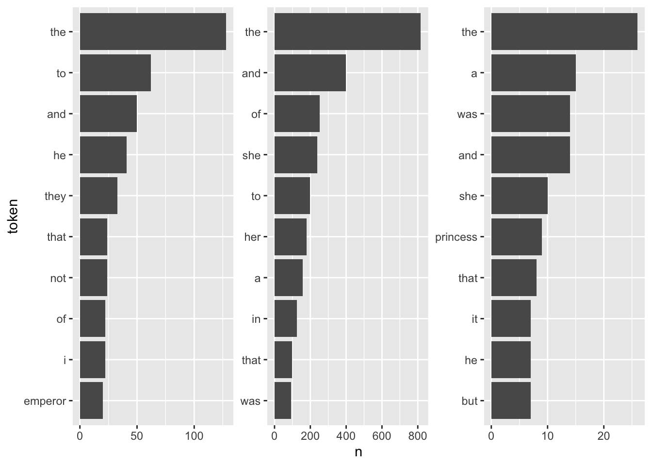

It is quite hard to draw inferences on which plot belongs to which book since the plots are crowded with stopwords. However, there are pre-made stopword lists I can harness to remove some of this “noise” and perhaps catch a bit more signal for determining the books.

# get_stopwords()
# stopwords_getsources()
# stopwords_getlanguages(source = "snowball")

fairytales_top10_nostop <- fairytales_tidy |> 
  anti_join(get_stopwords(), by = c("token" = "word")) |> 
  group_by(book) |> 
  count(token) |> 
  slice_max(n, n = 10, with_ties = FALSE)

fairytales_top10_nostop |> 
  ggplot()  +
  geom_col(aes(x = n, y = reorder_within(token, n, book))) +
  scale_y_reordered() +
  labs(y = "token") +
  facet_wrap(vars(book), scales = "free_y") +
  scale_x_continuous(breaks = scales::pretty_breaks()) +
  theme(strip.text.x = element_blank())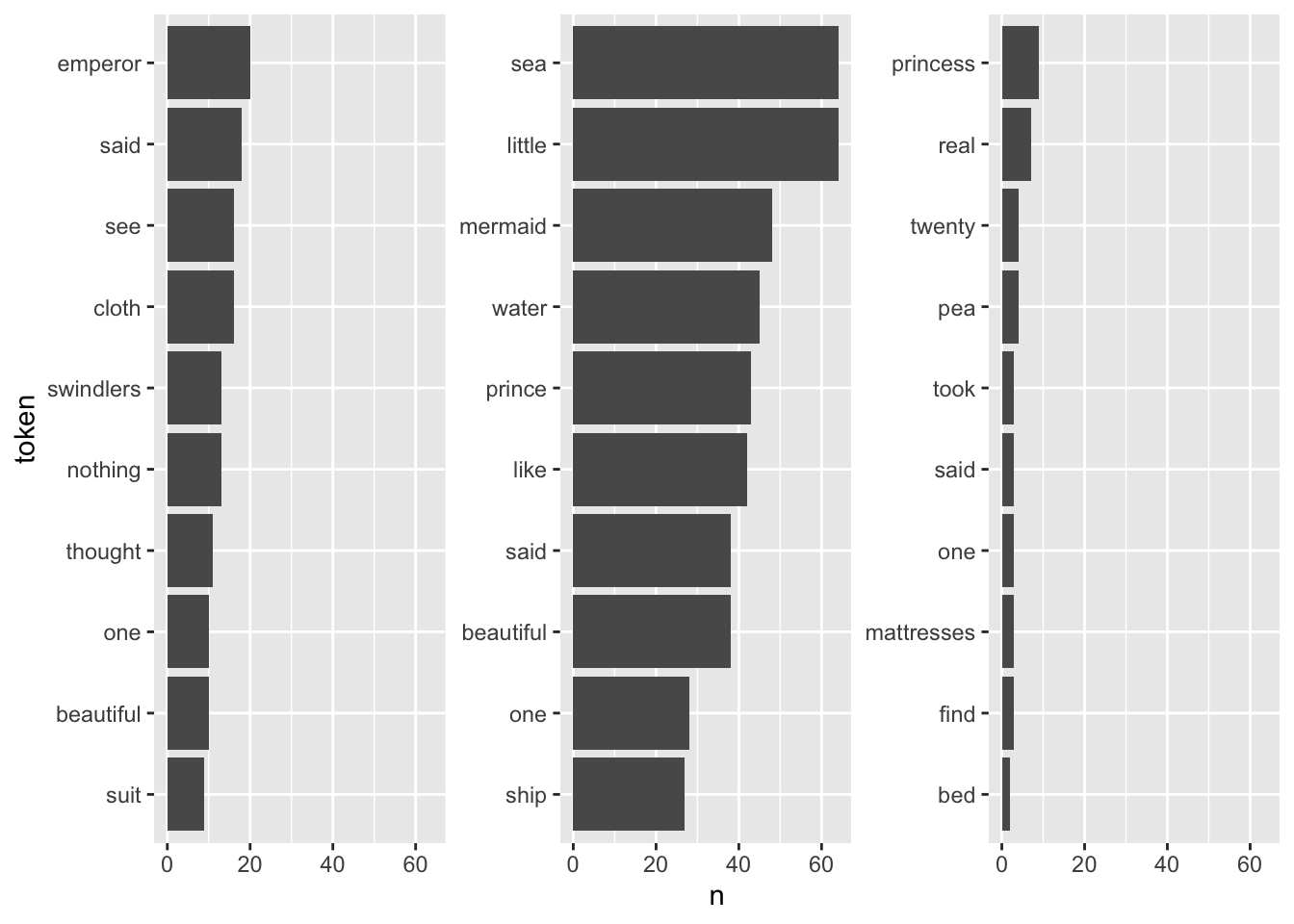

This already looks quite nice, it is quite easy to see which plot belongs to the respective book.

6.4.2 TF-IDF

A better definition of words that are particular to a group of documents is “the ones that appear often in one group but rarely in the other one(s)”. So far, the measure of term frequency only accounts for how often terms are used in the respective document. I can take into account how often it appears in other documents by including the inverse document frequency. The resulting measure is called tf-idf and describes “the frequency of a term adjusted for how rarely it is used.” (Silge and Robinson 2016: 31) If a term is rarely used overall but appears comparably often in a singular document, it might be safe to assume that it plays a bigger role in that document.

The tf-idf of a word in a document is commonly³. One implementation is calculated as follows:

\[w_{i,j}=tf_{i,j}\times ln(\frac{N}{df_{i}})\]

–> \(tf_{i,j}\): number of occurrences of term \(i\) in document \(j\)

–> \(df_{i}\): number of documents containing \(i\)

–> \(N\): total number of documents

Note that the \(ln\) is included so that words that appear in all documents – and do therefore not have discriminatory power – will automatically get a value of 0. This is because \(ln(1) = 0\). On the other hand, if a term appears in, say, 4 out of 20 documents, its ln(idf) is \(ln(20/4) = ln(5) = 1.6\).

The tidytext package provides a neat implementation for calculating the tf-idf called bind_tfidf(). It takes as input the columns containing the term, the document, and the document-term counts n.

fairytales_top10_tfidf <- fairytales_tidy |> 
  group_by(book) |> 
  count(token) |> 
  bind_tf_idf(token, book, n) |> 
  slice_max(tf_idf, n = 10)

fairytales_top10_tfidf |> 
  ggplot()  +
  geom_col(aes(x = tf_idf, y = reorder_within(token, tf_idf, book))) +
  scale_y_reordered() +
  labs(y = "token") +
  facet_wrap(vars(book), scales = "free") +
  theme(strip.text.x = element_blank(),
        axis.title.x = element_blank(),
        axis.text.x = element_blank(),
        axis.ticks.x = element_blank())

Pretty good already! All the fairytales can be clearly identified. A problem with this representation is that I cannot straightforwardly interpret the x-axis values (they can be removed by uncommenting the last four lines). A way to mitigate this is using odds.

Another shortcoming becomes visible when I take the terms with the highest TF-IDF as compared to all other fairytales.

tfidf_vs_full <- hcandersenr::hcandersen_en |> 
  unnest_tokens(output = token, input = text) |> 
  count(token, book) |> 
  bind_tf_idf(book, token, n) |> 
  filter(book %in% c("The princess and the pea",
                     "The little mermaid",
                     "The emperor's new suit")) 

plot_tf_idf <- function(df, group_var){
  df |> 
    group_by({{ group_var }}) |> 
    slice_max(tf_idf, n = 10, with_ties = FALSE) |> 
    ggplot()  +
    geom_col(aes(x = tf_idf, y = reorder_within(token, tf_idf, {{ group_var }}))) +
    scale_y_reordered() +
    labs(y = "token") +
    facet_wrap(vars({{ group_var }}), scales = "free") +
    #theme(strip.text.x = element_blank()) +
    theme(axis.title.x=element_blank(),
          axis.text.x=element_blank(),
          axis.ticks.x=element_blank())
} 
  
plot_tf_idf(tfidf_vs_full, book)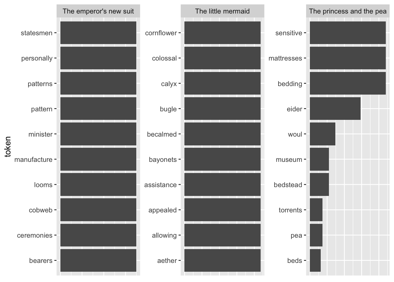

The tokens are far too specific to make any sense. Introducing a lower threshold (i.e., limiting the analysis to terms that appear at least x times in the document) might mitigate that. Yet, this threshold is of course arbitrary.

tfidf_vs_full |> 
  #group_by(token) |> 
  filter(n > 3) |> 
  ungroup() |> 
  plot_tf_idf(book)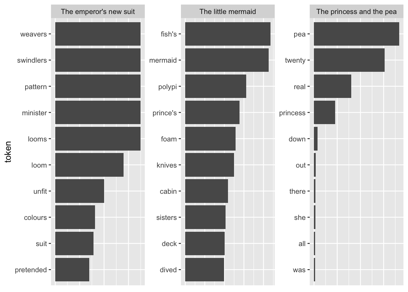

6.4.3 Exercises

3. Count the terms per party.

1. Do you see party-specific differences with regard to their ten most common terms (hint: slice_max(n, n = 10, with_ties = FALSE))?

df <- preprocessed |> 
  count(stemmed, party) |> 
  group_by(party) |> 
  slice_max(n, n = 10, with_ties = FALSE)
  
df |> 
  group_by(party) |> 
  ggplot()  +
    geom_col(aes(x = n, y = reorder_within(stemmed, n, party))) +
    scale_y_reordered() +
    labs(y = "token") +
    facet_wrap(vars(party), scales = "free") 

2. Is there more words you should add to your stopwords list? Remove these terms using filter(str_detect()) and a regex.

more_stopwords <- c("t.co", "http", "amp") 
df |> 
  filter(!str_detect(stemmed, str_c(more_stopwords, collapse = "|"))) |> 
  group_by(party) |> 
  ggplot()  +
    geom_col(aes(x = n, y = reorder_within(stemmed, n, party))) +
    scale_y_reordered() +
    labs(y = "token") +
    facet_wrap(vars(party), scales = "free") 

3. Do the same thing but using the spacy output and filtering only NOUNs and PROPNouns.

timelines_spacy |> 
  filter(pos %in% c("PROPN", "NOUN")) |> 
  left_join(timelines_meta |> 
              mutate(doc_id = as.character(doc_id)), by = "doc_id") |> 
  count(token, party) |>
  group_by(party) |> 
  slice_max(n, n = 10, with_ties = FALSE) |> 
  ggplot()  +
    geom_col(aes(x = n, y = reorder_within(token, n, party))) +
    scale_y_reordered() +
    labs(y = "token") +
    facet_wrap(vars(party), scales = "free") 

4. Again, is there stuff to be removed? Do so using a Regex.

timelines_spacy |> 
  filter(pos %in% c("PROPN", "NOUN"),
         !str_detect(token, "^@|[^a-z]|^amp$")) |> 
  left_join(timelines_meta |> 
              mutate(doc_id = as.character(doc_id)), by = "doc_id") |> 
  count(token, party) |>
  group_by(party) |> 
  slice_max(n, n = 10, with_ties = FALSE) |> 
  ggplot()  +
    geom_col(aes(x = n, y = reorder_within(token, n, party))) +
    scale_y_reordered() +
    labs(y = "token") +
    facet_wrap(vars(party), scales = "free") 

4. Do the same thing as in 3. but use TF-IDF instead of raw counts. How does this alter your results?

df_tf_idf <- preprocessed |> 
  count(word, party) |> 
  bind_tf_idf(word, party, n) |> 
  group_by(party) |> 
  slice_max(tf_idf, n = 10, with_ties = FALSE)
  
df_tf_idf |> 
  group_by(party) |> 
  ggplot()  +
    geom_col(aes(x = tf_idf, y = reorder_within(word, tf_idf, party))) +
    scale_y_reordered() +
    labs(y = "token") +
    facet_wrap(vars(party), scales = "free") 


timelines_spacy |> 
  #filter(pos %in% c("PROPN", "NOUN")) |> 
  left_join(timelines_meta |> 
              mutate(doc_id = as.character(doc_id)), by = "doc_id") |> 
  count(token, party) |>
  filter(str_detect(token, "[a-z]")) |> 
  filter(!str_detect(token, "^@")) |> 
  bind_tf_idf(token, party, n) |> 
  group_by(party) |> 
  slice_max(tf_idf, n = 10, with_ties = FALSE) |> 
  ggplot()  +
    geom_col(aes(x = tf_idf, y = reorder_within(token, tf_idf, party))) +
    scale_y_reordered() +
    labs(y = "token") +
    facet_wrap(vars(party), scales = "free") 

6.5 Dictionary-based Analysis

Sentiment analyses are fairly easy when you have your data in tidy text format. As they basically consist of matching the particular words’ sentiment values to the corpus, this can be done with an inner_join(). tidytext comes with four dictionaries: bing, loughran, afinn, and nrc:

walk(c("bing", "loughran", "afinn", "nrc"), ~get_sentiments(lexicon = .x) |> 
       head() |> 
       print())

# A tibble: 6 × 2
  word       sentiment
  <chr>      <chr>    
1 2-faces    negative 
2 abnormal   negative 
3 abolish    negative 
4 abominable negative 
5 abominably negative 
6 abominate  negative 
# A tibble: 6 × 2
  word         sentiment
  <chr>        <chr>    
1 abandon      negative 
2 abandoned    negative 
3 abandoning   negative 
4 abandonment  negative 
5 abandonments negative 
6 abandons     negative 
# A tibble: 6 × 2
  word       value
  <chr>      <dbl>
1 abandon       -2
2 abandoned     -2
3 abandons      -2
4 abducted      -2
5 abduction     -2
6 abductions    -2
# A tibble: 6 × 2
  word      sentiment
  <chr>     <chr>    
1 abacus    trust    
2 abandon   fear     
3 abandon   negative 
4 abandon   sadness  
5 abandoned anger    
6 abandoned fear     

As you can see here, the dictionaries are mere tibbles with two columns: “word” and “sentiment”. For easier joining, I should rename my column “token” to word.

needs(magrittr)
sotu_20cent_clean %<>% rename(word = token)

The AFINN dictionary is the only one with numeric values. You might have noticed that its words are not stemmed. Hence, I need to do this before I can join it with my tibble. To get the sentiment value per document, I need to average it.

sotu_20cent_afinn <- get_sentiments("afinn") |> 
  mutate(word = wordStem(word, language = "en")) |> 
  inner_join(sotu_20cent_clean) |> 
  group_by(year) |> 
  summarize(sentiment = mean(value))

Thereafter, I can just plot it:

sotu_20cent_afinn |> 
  ggplot() +
  geom_line(aes(x = year, y = sentiment))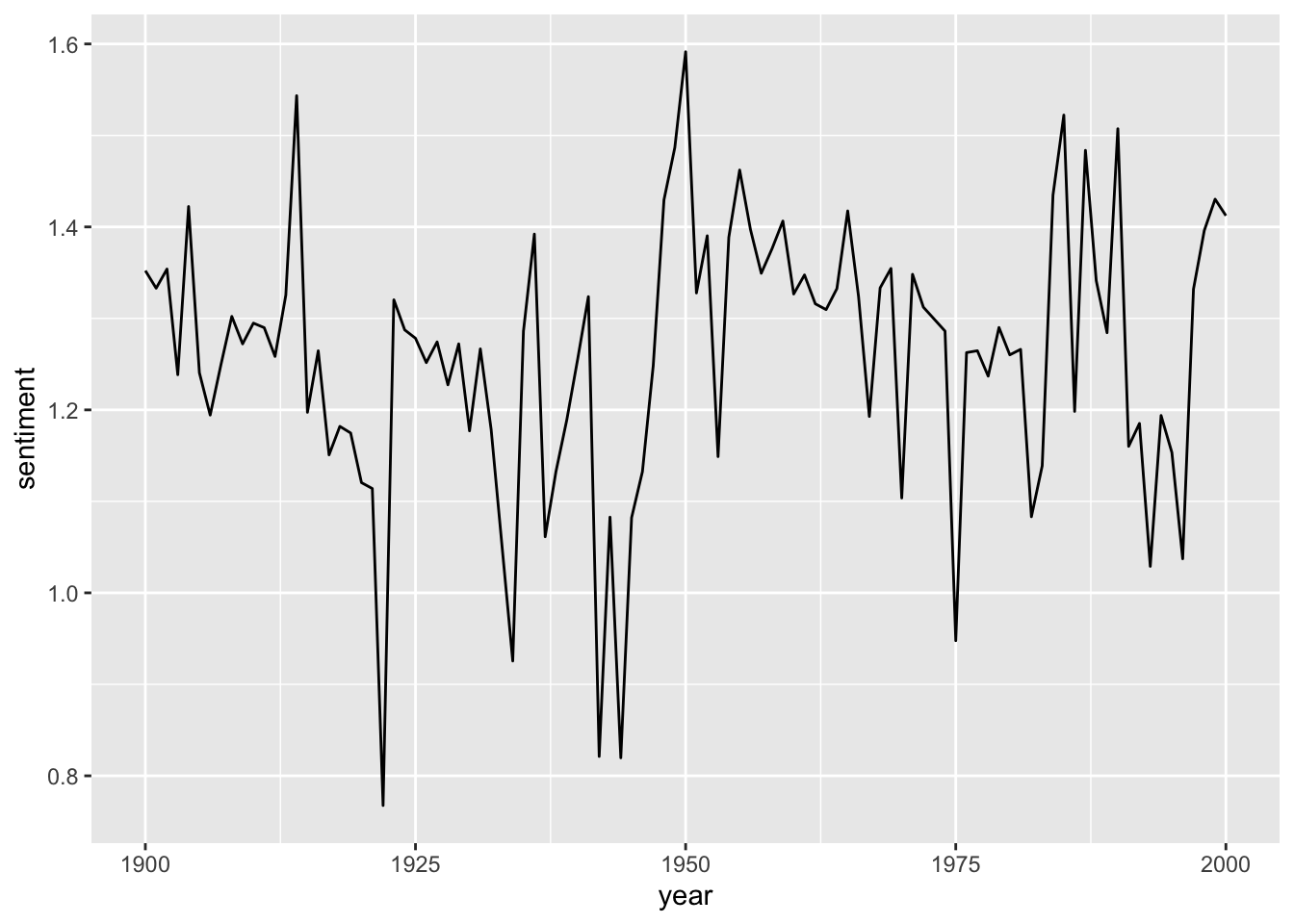

That’s a bit hard to interpret. geom_smooth() might help:

sotu_20cent_afinn |> 
  ggplot() +
  geom_smooth(aes(x = year, y = sentiment))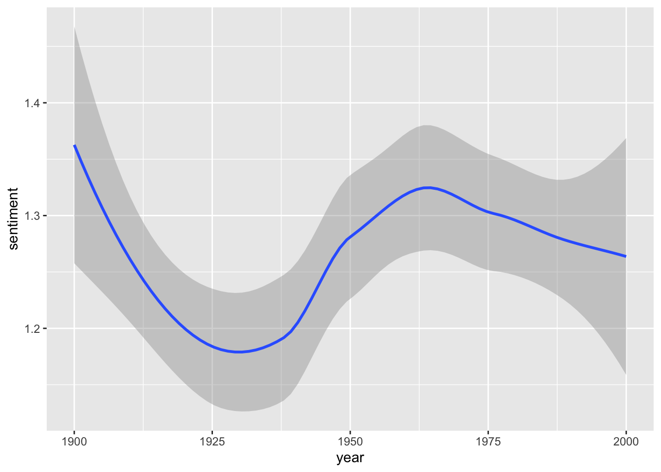

Interesting. When you think of the tone in the SOTU addresses as a proxy measure for the circumstances, the worst phase appears to be during the 1920s and 1930s – might make sense given the then economic circumstances, etc. The maximum was in around the 1960s and since then it has, apparently, remained fairly stable.

6.5.1 Assessing the results

However, we have no idea whether we are capturing some valid signal or not. Let’s look at what drives those classifications the most:

sotu_20cent_contribution <- get_sentiments("afinn") |> 
  mutate(word = wordStem(word, language = "en")) |> 
  inner_join(sotu_20cent_clean)  |>
  group_by(word) |>
  summarize(occurences = n(),
            contribution = sum(value))

sotu_20cent_contribution |>
  slice_max(contribution, n = 10) |>
  bind_rows(sotu_20cent_contribution |> slice_min(contribution, n = 10)) |> 
  mutate(word = reorder(word, contribution)) |>
  ggplot(aes(contribution, word, fill = contribution > 0)) +
  geom_col(show.legend = FALSE) +
  labs(y = NULL)

Let’s split this up per decade:

get_sentiments("afinn") |> 
  mutate(word = wordStem(word, language = "en")) |> 
  inner_join(sotu_20cent_clean) |>
  mutate(decade = ((year - 1900)/10) |> floor()) |>
  group_by(decade, word) |>
  summarize(occurrences = n(),
            contribution = sum(value)) |> 
  slice_max(contribution, n = 5) |>
  bind_rows(get_sentiments("afinn") |> 
              mutate(word = wordStem(word, language = "en")) |> 
              inner_join(sotu_20cent_clean) |>
              mutate(decade = ((year - 1900)/10) |> floor()) |>
              group_by(decade, word) |>
              summarize(occurrences = n(),
                        contribution = sum(value)) |> 
              slice_min(contribution, n = 5)) |> 
  mutate(word = reorder_within(word, contribution, decade)) |>
  ggplot(aes(contribution, word, fill = contribution > 0)) +
  geom_col(show.legend = FALSE) +
  facet_wrap(~decade, ncol = 4, scales = "free") +
  scale_y_reordered()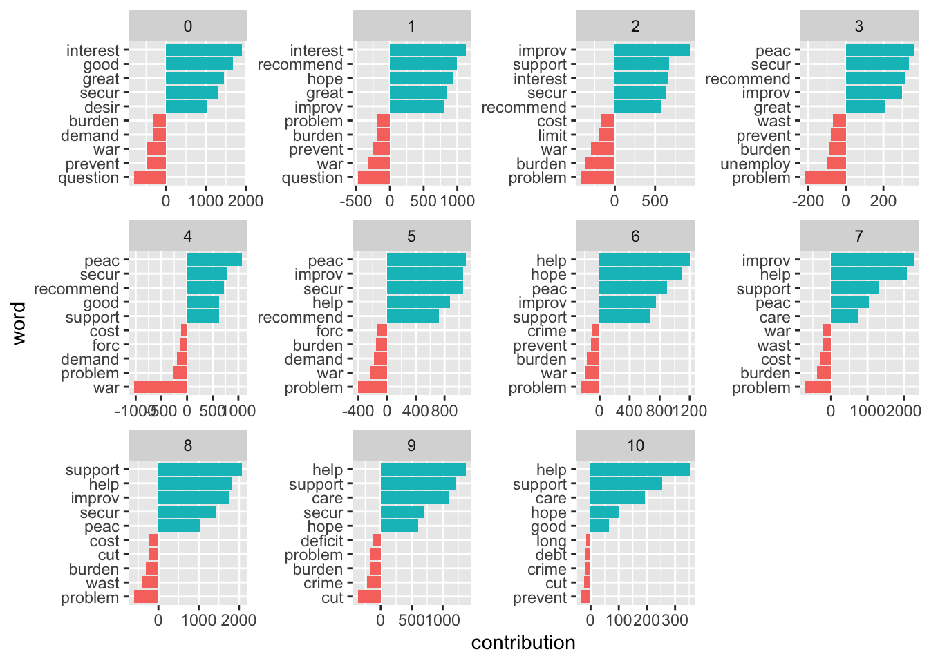

6.5.2 Assessing the quality of the rating

We need to assess the reliability of our classification (would different raters come to the same conclusion; and, if we compare it to a gold standard, how does the classification live up to its standards). One measure we can use here is Krippendorf’s Alpha which is defined as

\[\alpha = \frac{D_o}{D_e}\]

where \(D_{o}\) is the observed disagreement and \(D_{e}\) is the expected disagreement (by chance). The calculation of the measure is far more complicated, but R can easily take care of that – we just need to feed it with proper data. For this example I use a commonly used benchmark data set containing IMDb reviews of movies and whether they’re positive or negative.

imdb_reviews <- read_csv("https://www.dropbox.com/scl/fi/psgj6ze6at3zovildm728/imdb_reviews.csv?rlkey=ve2s02ydosbweemalvskyiu4s&dl=1")

glimpse(imdb_reviews)

Rows: 25,000
Columns: 2
$ text      <chr> "Once again Mr. Costner has dragged out a movie for far long…
$ sentiment <chr> "negative", "negative", "negative", "negative", "negative", …

imdb_reviews_afinn <- imdb_reviews |> 
  rowid_to_column("doc") |> 
  unnest_tokens(token, text) |> 
  anti_join(get_stopwords(), by = c("token" = "word")) |> 
  mutate(stemmed = wordStem(token)) |> 
  inner_join(get_sentiments("afinn") |> mutate(stemmed = wordStem(word))) |> 
  group_by(doc) |> 
  summarize(sentiment = mean(value)) |> 
  mutate(sentiment_afinn = case_when(sentiment > 0 ~ "positive",
                                     TRUE ~ "negative") |> 
           factor(levels = c("positive", "negative")))

Now we have two classifications, one “gold standard” from the data and the one obtained through AFINN.

review_coding <- imdb_reviews |> 
  mutate(true_sentiment = sentiment |> 
           factor(levels = c("positive", "negative"))) |> 
  select(-sentiment) |> 
  rowid_to_column("doc") |> 
  left_join(imdb_reviews_afinn |> select(doc, sentiment_afinn)) 

First, we can check how often AFINN got it right, the accuracy:

sum(review_coding$true_sentiment == review_coding$sentiment_afinn, na.rm = TRUE)/25000

[1] 0.64712

However, accuracy is not a perfect metric because it doesn’t tell you anything about the details. For instance, your classifier might just predict “positive” all of the time. If your gold standard has 50 percent “positive” cases, the accuracy would lie at 0.5. We can address this using the following measures.

For the calculation of Krippendorff’s Alpha, the data must be in a different format: a matrix containing with documents as columns and the respective ratings as rows.

needs(irr)
mat <- review_coding |> 
  select(-text) |> 
  as.matrix() |> 
  t()

mat[1:3, 1:5]

                [,1]       [,2]       [,3]       [,4]       [,5]      
doc             "    1"    "    2"    "    3"    "    4"    "    5"   
true_sentiment  "negative" "negative" "negative" "negative" "negative"
sentiment_afinn "positive" "negative" "negative" "positive" "positive"

colnames(mat) <- mat[1,]

mat <- mat[2:3,]
mat[1:2, 1:5]

                    1          2          3          4          5     
true_sentiment  "negative" "negative" "negative" "negative" "negative"
sentiment_afinn "positive" "negative" "negative" "positive" "positive"

irr::kripp.alpha(mat, method = "nominal")

 Krippendorff's alpha

 Subjects = 25000 
   Raters = 2 
    alpha = 0.266 

Good are alpha values of around 0.8 – AFINN missed that one.

Another way to evaluate the quality of classification is through a confusion matrix.

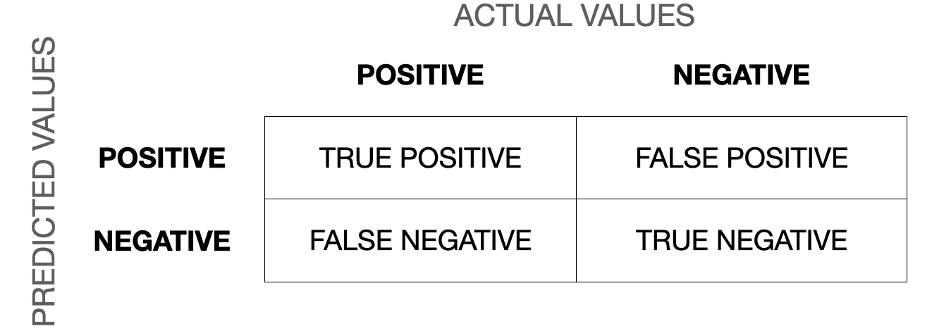
Now we can calculate precision (when it predicts “positive”, how often is it correct), recall/sensitivity (when it is “positive”, how often is this predicted), specificity (when it’s “negative”, how often is it actually negative). The F1-score is the harmonic mean of precision and recall and defined as \(F_1 = \frac{2}{\frac{1}{recall}\times \frac{1}{precision}} = 2\times \frac{precision\times recall}{precision + recall}\) and the most commonly used measure to assess the accuracy of the classification. The closer to 1 it is, the better. You can find a more thorough description of the confusion matrix and the different measures in this blog post.

We can do this in R using the caret package.

needs(caret)
confusion_matrix <- confusionMatrix(data = review_coding$sentiment_afinn, 
                                    reference = review_coding$true_sentiment,
                                    positive = "positive")
confusion_matrix$byClass

         Sensitivity          Specificity       Pos Pred Value 
           0.8439750            0.4504721            0.6056500 
      Neg Pred Value            Precision               Recall 
           0.7427441            0.6056500            0.8439750 
                  F1           Prevalence       Detection Rate 
           0.7052216            0.5000000            0.4219875 
Detection Prevalence    Balanced Accuracy 
           0.6967515            0.6472236 

6.5.3 Exercises

5. Take the abortion-related Tweets. Check for sentiment differences in parties. Use the AFINN dictionary. Plot your results.

sent_per_party <- preprocessed |> 
  inner_join(get_sentiments("afinn")) |> 
  mutate(word_sent = case_when(value > 0 ~ "positive",
                                value < 0 ~ "negative"))
sent_per_party |> 
  ggplot() +
  geom_bar(aes(word_sent)) +
  facet_wrap(vars(party))         
         
sent_per_doc <- preprocessed |> 
  inner_join(get_sentiments("afinn")) |> 
  group_by(doc_id, party) |> 
  summarize(mean_sent = mean(value)) |> 
  mutate(tweet_sent = case_when(mean_sent > 0 ~ "positive",
                                mean_sent < 0 ~ "negative",
                                TRUE ~ "neutral"))

sent_per_doc |> 
  ggplot() +
  geom_bar(aes(tweet_sent)) +
  facet_wrap(vars(party))

6. Have a look at different dictionaries (e.g., Bing or Loughran). Check the words that contributed the most. Do you see any immediate ambiguities or flaws?

# afinn
tweets_abortion_tidy_contribution_afinn <- preprocessed |> 
  inner_join(get_sentiments("afinn")) |> 
  group_by(party, word) |>
  summarize(contribution = sum(value))

bind_rows(
  tweets_abortion_tidy_contribution_afinn |> 
    filter(party == "D") |> 
    slice_max(contribution, n = 10, with_ties = FALSE) |> 
    mutate(type = "pos"),
  tweets_abortion_tidy_contribution_afinn |> 
    filter(party == "D") |> 
    slice_min(contribution, n = 10, with_ties = FALSE) |> 
    mutate(type = "neg"),
  tweets_abortion_tidy_contribution_afinn |> 
    filter(party == "R") |> 
    slice_max(contribution, n = 10, with_ties = FALSE) |> 
    mutate(type = "pos"),
  tweets_abortion_tidy_contribution_afinn |> 
    filter(party == "R") |> 
    slice_min(contribution, n = 10, with_ties = FALSE) |> 
    mutate(type = "neg")
) |> 
  mutate(word = reorder_within(word, contribution, party)) |>
  ggplot() +
  geom_col(aes(contribution, word), show.legend = FALSE) +
    scale_y_reordered() +
    facet_wrap(vars(party, type), scales = "free")

# loughran
needs(ggpubr)

tweets_abortion_tidy_contribution_loughran <- preprocessed |> 
  inner_join(get_sentiments("loughran")) |> 
  count(party, sentiment, word) |> 
  group_by(party, sentiment) |> 
  slice_max(n, n = 10, with_ties = FALSE) |> 
  group_split()

tweets_abortion_tidy_contribution_loughran |> 
  map(\(x) x |> 
        mutate(word = reorder_within(word, n, party)) |> 
        slice_max(n, n = 10) |> 
        ggplot() +
        geom_col(aes(n, word), show.legend = FALSE) +
        scale_y_reordered() +
        labs(title = x[["sentiment"]][1])
  ) |> 
  ggarrange(plotlist = _)
  
# bing
tweets_abortion_tidy_contribution_bing <- preprocessed |> 
  inner_join(get_sentiments("bing")) |> 
  count(party, sentiment, word) |> 
  group_by(party, word, sentiment) |> 
  summarize(contribution = sum(n)) |> 
  group_by(party, sentiment) |> 
  slice_max(contribution, n = 10, with_ties = FALSE) |> 
  mutate(contribution = case_when(
    sentiment == "negative" ~ contribution * (-1),
    TRUE ~ contribution
  ))

tweets_abortion_tidy_contribution_bing |> 
  mutate(word = reorder_within(word, contribution, party)) |>
  ggplot() +
  geom_col(aes(contribution, word), show.legend = FALSE) +
    scale_y_reordered() +
    facet_wrap(vars(party, sentiment), scales = "free")

6.6 Further links

• Tidy text mining with R.
• A more general introduction by Christopher Bail.
• A guide to Using spacyr.

Benoit, Kenneth, and Akitaka Matsuo. 2020. “Spacyr: Wrapper to the ’spaCy’ ’NLP’ Library.”

Benoit, Kenneth, Kohei Watanabe, Haiyan Wang, Paul Nulty, Adam Obeng, Stefan Müller, and Akitaka Matsuo. 2018. “Quanteda: An R Package for the Quantitative Analysis of Textual Data.” Journal of Open Source Software 3 (30): 774. https://doi.org/10.21105/joss.00774.

Feinerer, Ingo, Kurt Hornik, and David Meyer. 2008. “Text Mining Infrastructure in R.” Journal of Statistical Software 25 (5). https://doi.org/10.18637/jss.v025.i05.

Grimmer, Justin, Margaret Roberts, and Brandon Stewart. 2022. Text as Data: A New Framework for Machine Learning and the Social Sciences. Princeton: Princeton University Press.

Honnibal, Matthew, and Ines Montani. 2017. “spaCy 2: Natural Language Understanding with Bloom Embeddings, Convolutional Neural Networks and Incremental Parsing.”

Manning, Christopher D, Prabhakar Raghavan, and Hinrich Schütze. 2008. Introduction to Information Retrieval. New York: Cambridge University Press.

Monroe, Burt L., Michael P. Colaresi, and Kevin M. Quinn. 2008. “Fightin’ Words: Lexical Feature Selection and Evaluation for Identifying the Content of Political Conflict.” Political Analysis 16 (4): 372–403. https://doi.org/10.1093/pan/mpn018.

Silge, Julia, and David Robinson. 2016. “Tidytext: Text Mining and Analysis Using Tidy Data Principles in R.” The Journal of Open Source Software 1 (3): 37. https://doi.org/10.21105/joss.00037.

---

1. Each observation has its own row, each variable its own column, each value has its own cell, find more here

2. overview copied from the webpage

3. Note that multiple implementations exist, for an overview see, for instance, Manning, Raghavan, and Schütze (2008)