Chapter 5 Mapping Vector Data
5.1 Map point vector data of superfund sites
Alrighty! Now our data seems to be prepared and we can move on to mapping our data.
First things first, this website will be extremely useful in producing leaflet maps : https://rstudio.github.io/leaflet/.
Let's map the superfund sites.
Start by calling leaflet()- this tells R that we want to create an interactive map using the leaflet package. Next, we want to add a basemap (a background). To do this, we tell R addTiles(). Note: the %>% symbols tell R to add another layer to the map.
Now, we have an interactive map interface and a background map. Naturally, the next step is actually adding our data to the top of the map. Before we add our data to the map we have to consider: What type of data is our superfund dataset? In this case, it's point vector data, where each point represents the location of a superfund site. We use the function addMarkers() to add point data to the leaflet map.
leaflet() %>%
addTiles() %>%
addMarkers(data = superfund_projected)What if we want to add other data types other than point vector data? We just need to change the function name that calls the data.
addMarkers()adds point vector data
addPolylines()adds line data
addPolygons()adds polygon data
addRasterImage()adds raster data to a map.
5.2 Map polygon vector data of the social vulnerability index
Now, let's try a more complex example. Let's try to map the social vulnerability index data. First, let's start by initializing our leaflet map and adding a basemap to it: leaflet() %>% addTiles(). Next, we add our social vulnerability data as a layer to the map. Again, let's reflect what type of data the social vulnerability index is... So, the social vulnerability index is an aggregated dataset. Each census track gets a value from 0 (no vulnerability) to 1 (high vulnerability) representing the social vulnerability of that census track area. So now we know that this dataset is areal- this means that it cannot be a point or line type of data and it can only be represented by polygons. Therefore, we use addPolygons() to add our SVI dataset.
leaflet() %>% addTiles() %>%
addPolygons(data = svi_projected) Our SVI map is plotted, but it doesn't quite look right. This is because the default for mapping polygons is plotting the borders. R doesn't automatically know what you want to see in your map. Here, we want to visualize the difference in social vulnerability across the area. So let's look into our svi dataset and see what features we have using the function names().
names(svi_projected)## [1] "svi_overall" "svi_socioeconomic" "svi_homecomposition"
## [4] "svi_minority" "svi_housingaccess"So we have 5 features:
- svi_overall: this designates the overall social vulnerability
- svi_socioeconomic: this represents social vulnerability by considering only socioeconomic status
- svi_homecomposition: this represents the social vulnerbaility considering only household composition and disability status
- svi_minority: this represents the social vulnerbility considering only minority status and english speaking ability
- svi_housingaccess: lastly this showcases the vulnerability associated with/without access to housing and transportation
We want to make a plot showing the overall social vulnerability. Let's do this! First things first, let's make a color palette for our map. We want a continous color ramp for our overall social vulnerbaility index values, where 0 is white and 1 is dark red. This would be appropriate because the more red the polygons get, then the more socially vulnerabile those areas are. Note: you can run the code colors() to view all the colors that R knows by name.
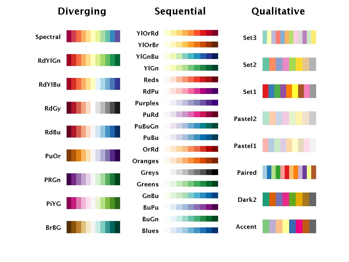
Here, we want a nice color palette. The R package RColorBrewer has great color palette options, as shown below. Here, we are going to use the "Reds" color palette to represent the range of social vulnerbaility values. The function colorBin() below creates a continuous color ramp of 5 different colors ranging across white to red that span the values for our overall social vulnerability index.
library(RColorBrewer)
pal <- colorBin(palette = "Reds",
domain = svi$svi_overall, n = 5) # split colors from white to red into 9 even bins
leaflet() %>% addTiles() %>%
addPolygons(data = svi_projected,
label= ~svi_overall, # when you hover over the polygon, it will label the svi
color = "gray", # the color of the border
fillColor = ~pal(svi_projected$svi_overall), # the colors inside the polygons
weight = 1.0, # the thickness of the border lines
opacity = 1.0, # the transparency of the border lines
fillOpacity = 0.8) # the transparency inside the polygonsNow this is a much better looking map. Let's go ahead and add a legend to the map as well. To designate a legend, we add a legend layer to the leaflet map using addLegend(). Within the addLegend() function we can provide a number of arguments to create a nice looking legend: the dataset's variable name, the location of the legend, the color palette we used to visualize our data, the attribute we used to vizualize our dataset, the title of our legend, and the opacity of the legend.
leaflet() %>% addTiles() %>%
addPolygons(data = svi_projected,
label= ~svi_overall, # when you hover over the polygon, it will label the svi
color = "gray", # the color of the border
fillColor = ~pal(svi_projected$svi_overall), # the colors inside the polygons
weight = 1.0, # the thickness of the border lines
opacity = 1.0, # the transparency of the border lines
fillOpacity = 0.8) %>% # the transparency inside the polygons
addLegend(data= svi_projected, # the dataset
"bottomright", # where to put the legend
pal=pal, values = ~svi_overall, # specify the color palette and the range of values
title="SVI", # legend title
opacity = 1.0) # the transparency of the legend