Chapter 7 Mapping Exercise

Now let's conduct an example where we download GIS data from a repository and map it. So let's download two geospatial datasets and create a map with those two layers. First, visit http://www.gis.pr.gov/descargaGeodatos/Pages/default.aspx and click on "Conservación", as shown below.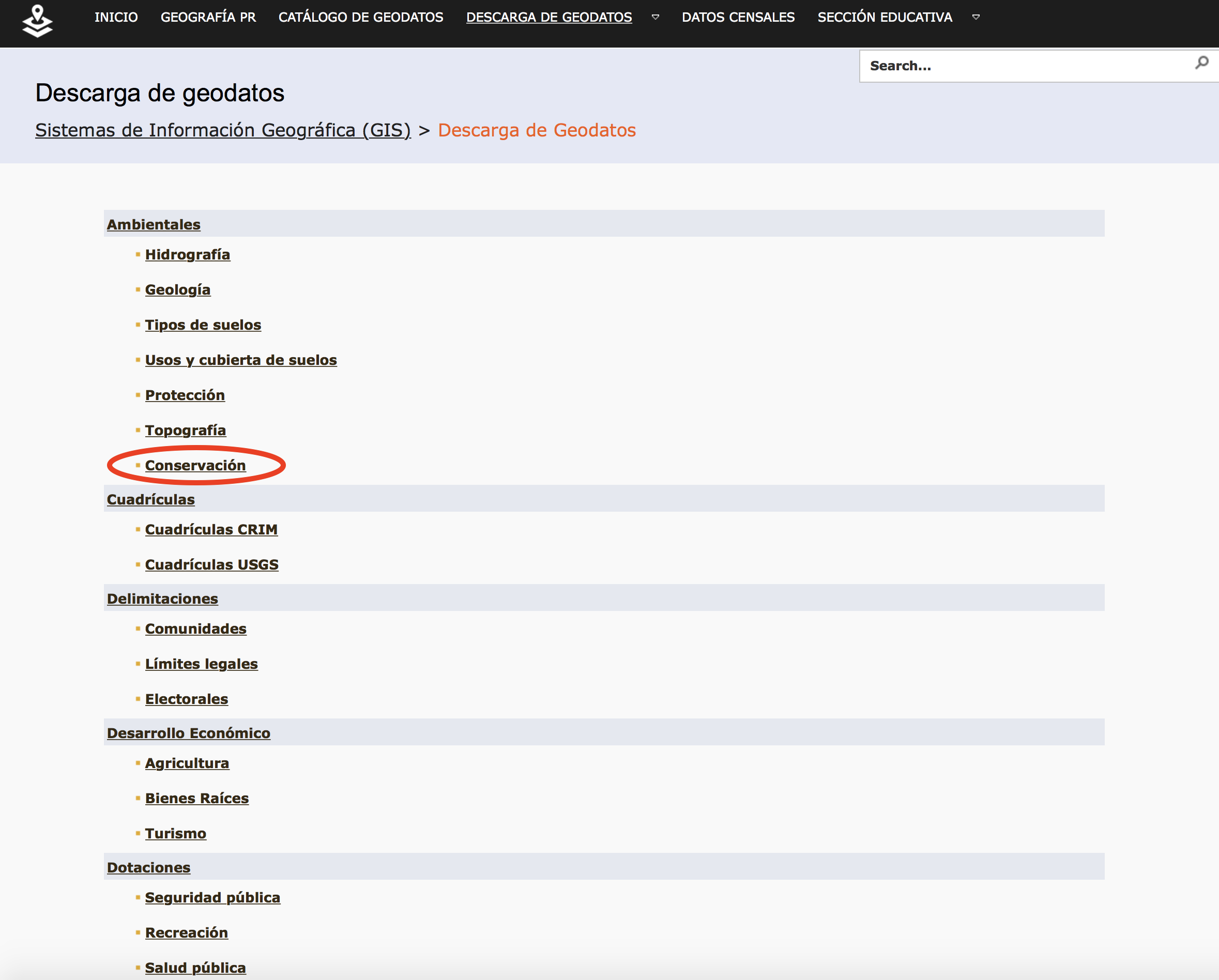

Next, click on "Critical wildlife areas" to download a shapefile of the critical wildlife areas in Puerto Rico. Save the data into a folder named "wildlife" and import the data using the following functions:

# Import our libraries to import the data (rgdal) and then map the data (leaflet) 
library(rgdal) # contains functions for importing and wrangling vector data
library(leaflet) # contains functions for mapping our data 

wildlife_dir <- "~/Desktop/wildlife/critical_wildlife_areas.shp"
wildlife <- readOGR(wildlife_dir)

## OGR data source with driver: ESRI Shapefile 
## Source: "/Users/eminefidan/Desktop/wildlife/critical_wildlife_areas.shp", layer: "critical_wildlife_areas"
## with 225 features
## It has 13 fields

Let's go ahead and download another dataset for mapping by visiting this GIS data repository. Next, find and click on the Download button and select "Shapefile" to download the dataset. Go ahead and import this dataset into R:

hospitals_dir <- "~/Downloads/Hospitals-shp/Hospitals.shp"
hospitals <- readOGR(hospitals_dir)

## OGR data source with driver: ESRI Shapefile 
## Source: "/Users/eminefidan/Downloads/Hospitals-shp/Hospitals.shp", layer: "Hospitals"
## with 7596 features
## It has 32 fields

Now that the data is imported into R, we should check the coordinate system and project it to a geographic coordinate system that leaflet prefers. The code below demonstrates this:

crs(wildlife)

## CRS arguments:
##  +proj=lcc +lat_0=17.8333333333333 +lon_0=-66.4333333333333
## +lat_1=18.4333333333333 +lat_2=18.0333333333333 +x_0=200000 +y_0=200000
## +ellps=GRS80 +units=m +no_defs

crs(hospitals)

## CRS arguments:
##  +proj=merc +a=6378137 +b=6378137 +lat_ts=0 +lon_0=0 +x_0=0 +y_0=0 +k=1
## +units=m +nadgrids=@null +wktext +no_defs

new_crs <- '+init=epsg:4326' 
wildlife_projected <- spTransform(wildlife, CRS(new_crs))
hospitals_projected <- spTransform(hospitals, CRS(new_crs))

# Double check the new projection of our data
crs(wildlife_projected)

## CRS arguments: +proj=longlat +datum=WGS84 +no_defs

crs(hospitals_projected)

## CRS arguments: +proj=longlat +datum=WGS84 +no_defs

If we aren't sure what type of vector data our GIS datasets are, then we can we the plot() function to generate a basic plot of our data. Within the plot function we provide the variable name of our dataset.

plot(wildlife_projected)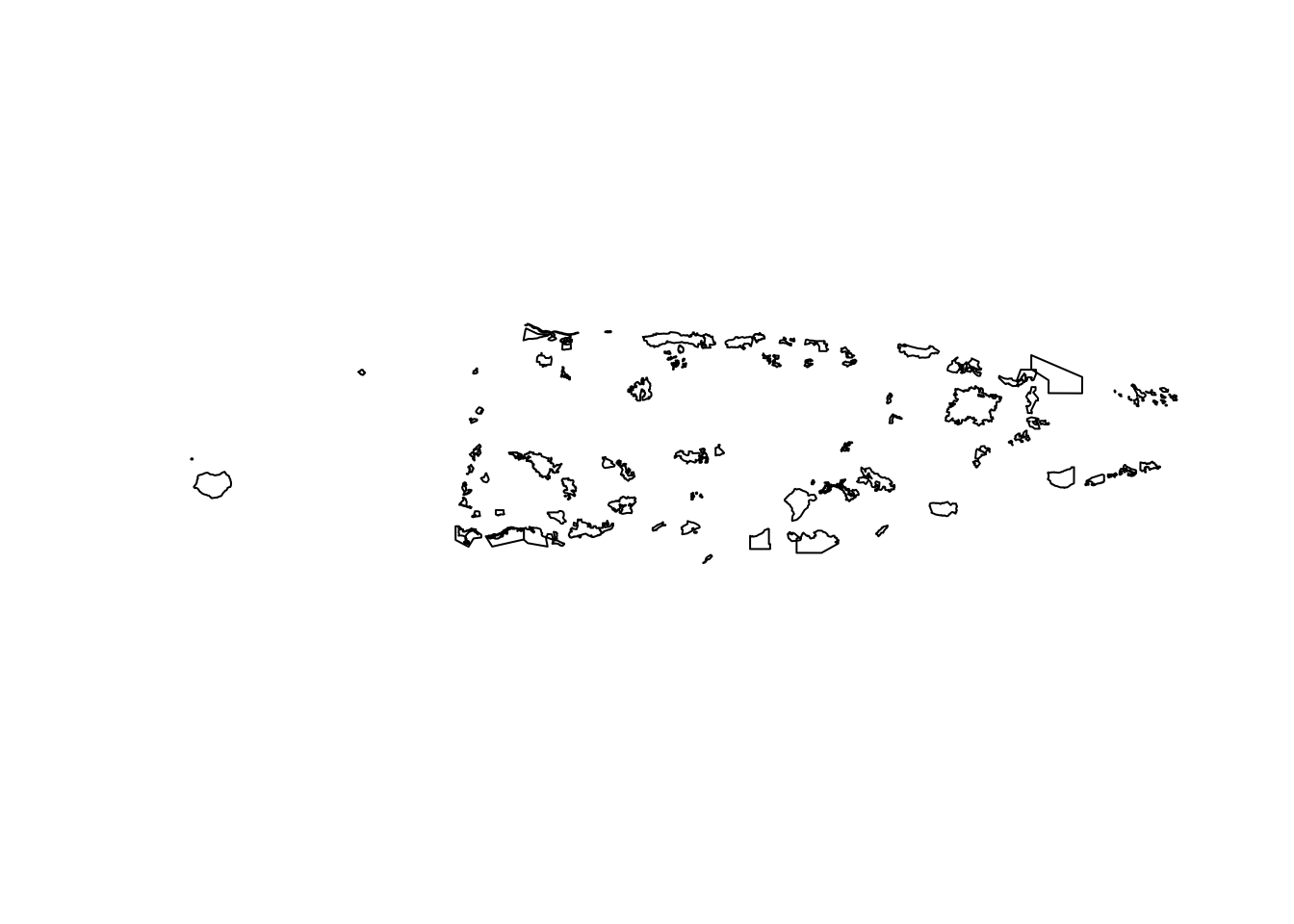

plot(hospitals_projected)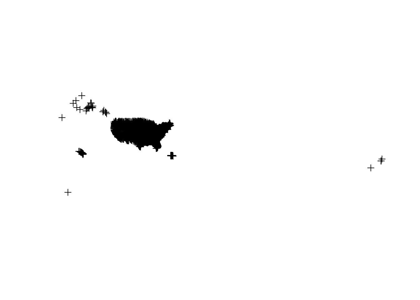

Although these plots aren't very pretty, it gives us some good information regarding the data type. From this figure, it is apparent that the critical wildlife areas dataset is a polygon vector data type and the hospitals dataset is a point vector data type. Thus, our next step is to create our leaflet map using the addPolygons() and addCircleMarkers() functions.

leaflet() %>% addTiles() %>% 
  addPolygons(data = wildlife_projected) %>% 
  addCircleMarkers(data = hospitals_projected)

Great! Our map is created! Now, let's spice it up by changing the appearance. First things first, we only want to view information in Puerto Rico, so let's zoom into the center of Puerto Rico on the map using the setView() function and specifying the center of our map and the zoom level. By Googling coordinates of Puerto Rico, I found this: (-66.480856, 18.224794) where -66.48 is the longitude coordinate and 18.22 is the latitude coordinate. So when I set the view of the leaflet map, I will need to specify the longitude coordinate of the center of the map, latitude of the center of the map, and the zoom level (which I picked as 9 since that seemed to fit the country's extent the best).
For the polygon data:
We can change the color of the border and the inside of the area using the options color and fillColor, respectively, and providing any color name (you can see what color names R recognizes using colors() function). Additionally, we can change the thickness of our border line using weight and changing it to any value we see fit. Next, we can set the transparency of our border and polygon area using the functions opacity and fillOpacity, respectively. Values for opacity can range from 0 to 1, where 0 indicates complete transparency and 1 indicates complete opaqueness. Lastly, here I add the option highlightOptions = highlightOptions(color = "white", weight = 2, bringToFront = TRUE), which highlights any polygon that my cursor hovers over. These options are highlighted in our reference content.
For the point data:
We can change the size of our markers by specifying the radius option. Similar to the polygon data, the color, weight, and fillOpacity parameters can be specified as well. We can even add pop-up labels to each point using popup so that information pops up when we click on an hospital marker. When specifying the information that you want to pop-up, you need to designate the specific name of an attribute in your dataset's attribute table. So here, I ran the code names(hospitals_projected) to get back the attribute names available for the hospitals dataset. NAMES is an attribute on the attribute table that specifies the name of the hospital, so if I want this attribute to be display when I click on a point then I need to add pop = ~NAME as an argument in the code.

leaflet() %>% addTiles() %>% 
  addPolygons(data = wildlife_projected, 
              color = "forestgreen",
              fillColor = "forestgreen",
              weight = 1.0,
              opacity = 0.9, 
              fillOpacity = 0.5,
              highlightOptions = highlightOptions(color = "white", weight = 2, bringToFront = TRUE)) %>% 
  addCircleMarkers(data = hospitals_projected,
                   color = "tomato",
                   fillColor = "red",
                   radius = 5.0,
                   weight = 1.0, 
                   fillOpacity = 0.8,
                   popup = ~NAME) %>% 
  setView(lng = -66.48, lat = 18.22, zoom = 9)