8  Least Squares and Applications

The Least Squares method is a foundational statistical technique used to model the relationship between variables and predict outcomes. By minimizing the sum of squared differences between observed data points and the values predicted by a model, it ensures the best fit for a given dataset. This approach is widely applied across various fields such as data analysis, engineering, economics, and machine learning.

This document explores the Least Squares method, focusing on its application in linear regression. Practical examples in Python are provided to demonstrate how to implement this method and interpret results effectively.

8.1 Least Squares Method

The Least Squares Method is a statistical technique used to find the best-fitting line through a set of data points. In the context of simple linear regression, this method is used to minimize the sum of squared differences between the observed data points and the predicted values by the model.

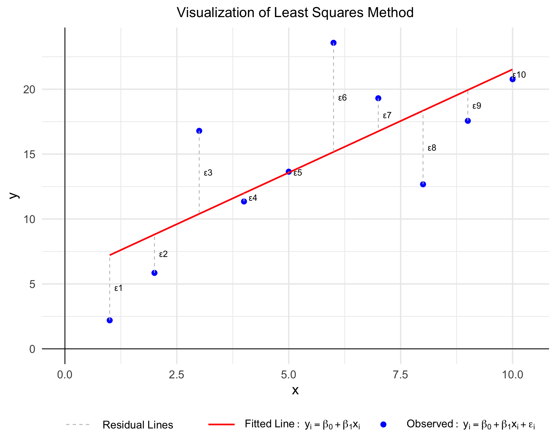
8.2 Linear Regression Model and Matrix Equation

In simple linear regression, we aim to find a line that best fits the data. Let’s consider we have a dataset with $n$ data points $(x_1,y_1),(x_2,y_2),\dots ,(x_n,y_n)$. The linear regression model is represented as:

$$y_i={\beta }_0+{\beta }_1{x}_i+{ϵ}_i$$

Where:

• $y_i$ is the observed value,
• $x_i$ is the predictor (independent variable),
• ${\beta }_0$ is the intercept,
• ${\beta }_1$ is the slope of the line,
• ${ϵ}_i$ is the residual (error term) for each data point.

We can write this equation for all data points in a vector and matrix form as:

$$\begin{array}{rl}Y& =\beta X+ϵ\\ & =\left[\begin{array}{c}{\beta }_0\\ ⋮\\ {\beta }_{(n-1)}\end{array}\right]\left[\begin{array}{cc}1& x_1\\ 1& x_2\\ ⋮\\ 1& x_n\end{array}\right]+\left[\begin{array}{c}{ϵ}_1\\ {ϵ}_2\\ ⋮\\ {ϵ}_n\end{array}\right]\end{array}$$

8.3 Finding the Coefficients $\beta$ Using Least Squares

In linear regression, the primary objective is to find the best-fitting line that represents the relationship between the independent variable ($X$) and the dependent variable ($Y$). To measure how well the line fits the data, we use the concept of the Residual Sum of Squares (RSS).

Residuals ($ϵ$) are the differences between the actual values ($Y$) and the predicted values from the model ($X\beta$), expressed as:

$$ϵ=Y-X\beta$$

The RSS is calculated by summing the squared residuals across all data points, which gives the formula:

$$\begin{array}{rl}RSS& =\sum _{i=1}^n{ϵ}_i^2\\ & =\parallel Y-X\beta {\parallel }^2\end{array}$$

Expanding this residual sum of squares (RSS) as:

$$RSS=(Y-X\beta {)}^T(Y-X\beta )$$

Expanding this quadratic form:

$$RSS=Y^{T}Y-2{\beta }^T{X}^{T}Y+{\beta }^T{X}^{T}X\beta$$

where:

• $Y^{T}Y$ is a scalar resulting from the dot product of $Y$ with itself.
• $-2{\beta }^T{X}^{T}Y$ is the cross-term representing the interaction between predictors and the response.
• ${\beta }^T{X}^{T}X\beta$ is the quadratic term involving the coefficients $\beta$.

To minimize $RSS$, differentiate with respect to $\beta$:

$$\frac{\partial RSS}{\partial \beta }=\frac{\partial }{\partial \beta }(Y^{T}Y-2{\beta }^T{X}^{T}Y+{\beta }^T{X}^{T}X\beta )$$

The derivatives are:

• $\frac{\partial }{\partial \beta }(Y^{T}Y)=0$, as $Y^{T}Y$ is independent of $\beta$.
• $\frac{\partial }{\partial \beta }(-2{\beta }^T{X}^{T}Y)=-2X^{T}Y$.
• $\frac{\partial }{\partial \beta }({\beta }^T{X}^{T}X\beta )=2X^{T}X\beta$.

Combining these: $$\frac{\partial RSS}{\partial \beta }=-2X^{T}Y+2X^{T}X\beta$$

To find the value of $\beta$ that minimizes $RSS$, set the derivative to zero:

$$-2X^{T}Y+2X^{T}X\beta =0$$

Simplify:

$$X^{T}X\beta =X^{T}Y$$

8.4 Solving the Normal Equation

To find $\beta$, we solve the normal equation:

$$\beta =(X^{T}X{)}^{-1}{X}^{T}Y$$

This gives us the values of the coefficients ${\beta }_0$ and ${\beta }_1$ (or other coefficients in a more complex model). This solution involves matrix operations, such as matrix multiplication and matrix inversion.

8.5 Linear Regression Example

8.5.1 Data

We have the following data:

x	y
1	2.197622
2	5.849113
3	16.793542
4	11.352542
5	13.646439
6	23.575325
7	19.304581
8	12.674694
9	17.565736
10	20.771690

Python can be applied to generate data as the following code:

import numpy as np
import pandas as pd

# Set seed for reproducibility
np.random.seed(123)

# Create the data
x = np.arange(1, 11)
y = 2 * x + 3 + np.random.normal(0, 5, 10)

# Create a DataFrame
data = pd.DataFrame({'x': x, 'y': y})

# Display the data
print(data)

set.seed(123)
x <- 1:10
y <- 2 * x + 3 + rnorm(10, mean = 0, sd = 5)
data <- data.frame(x, y)

# Display the data
data

    x         y
1   1  2.197622
2   2  5.849113
3   3 16.793542
4   4 11.352542
5   5 13.646439
6   6 23.575325
7   7 19.304581
8   8 12.674694
9   9 17.565736
10 10 20.771690

8.5.2 Linear Regression Equation

The linear regression model for this data can be written as:

$$y_i={\beta }_0+{\beta }_1{x}_i+{ϵ}_i$$

Where

• $y_i$ is the predicted value,
• $x_i$ is the input data,
• ${\beta }_0$ is the intercept,
• ${\beta }_1$ is the slope, and
• ${ϵ}_i$ is the error.

8.5.3 Matrix $\mathbf{X}$ and Vector $\mathbf{y}$

Create matrix $\mathbf{X}$, which consists of the first column of ones for the intercept and the second column containing the data $x_i$, and vector $\mathbf{y}$ containing the values $y_i$.

import numpy as np

# Assuming data is already defined as a pandas DataFrame
X = np.column_stack((np.ones(len(data)), data['x']))  # Add a column of ones for the intercept
y = data['y'].values  # Convert the 'y' column to a numpy array

# Display X and y
print("X:\n", X)
print("y:\n", y)

# Matrix X and vector y
X <- cbind(1, data$x)  # Add a column of ones for the intercept
y <- data$y

X

      [,1] [,2]
 [1,]    1    1
 [2,]    1    2
 [3,]    1    3
 [4,]    1    4
 [5,]    1    5
 [6,]    1    6
 [7,]    1    7
 [8,]    1    8
 [9,]    1    9
[10,]    1   10

y

 [1]  2.197622  5.849113 16.793542 11.352542 13.646439 23.575325 19.304581
 [8] 12.674694 17.565736 20.771690

8.5.4 Compute ${\mathbf{X}}^T\mathbf{X}$

Next, we compute ${\mathbf{X}}^T\mathbf{X}$:

$${\mathbf{X}}^T\mathbf{X}=\left[\begin{array}{cc}\sum 1& \sum x_i\\ \sum x_i& \sum x_i^2\end{array}\right]$$

import numpy as np

# Assuming X is already defined as a numpy array
X_t_X = np.dot(X.T, X)

# Display the result
print(X_t_X)

# Compute X'X
X_t_X <- t(X) %*% X
X_t_X

     [,1] [,2]
[1,]   10   55
[2,]   55  385

8.5.5 Compute ${\mathbf{X}}^T\mathbf{y}$

Now, we compute ${\mathbf{X}}^T\mathbf{y}$:

$${\mathbf{X}}^T\mathbf{y}=\left[\begin{array}{c}\sum y_i\\ \sum x_i{y}_i\end{array}\right]$$

# Compute X'Y
X_t_y = np.dot(X.T, y)

# Display the result
print(X_t_y)

# Compute X'Y
X_t_y <- t(X) %*% y
X_t_y

         [,1]
[1,] 143.7313
[2,] 921.7089

8.5.6 Compute the Inverse of ${\mathbf{X}}^T\mathbf{X}$

To compute $({\mathbf{X}}^T\mathbf{X}{)}^{-1}$, we use the matrix inverse function:

# Compute the inverse of X'X
inv_X_t_X = np.linalg.inv(X_t_X)

# Display the result
print(inv_X_t_X)

# Compute the inverse of X'X
inv_X_t_X <- solve(X_t_X)
inv_X_t_X

            [,1]        [,2]
[1,]  0.46666667 -0.06666667
[2,] -0.06666667  0.01212121

8.6 7. Compute the Vector $\mathit{\beta }$

Now we can compute the vector $\mathit{\beta }$:

$$\mathit{\beta }=({\mathbf{X}}^T\mathbf{X}{)}^{-1}{\mathbf{X}}^T\mathbf{y}$$

# Compute the beta vector
beta = np.dot(inv_X_t_X, X_t_y)

# Display the result
print(beta)

# Compute the beta vector
beta <- inv_X_t_X %*% X_t_y
beta

         [,1]
[1,] 5.627337
[2,] 1.590144

8.7 8. Linear Regression Equation

Thus, the estimated regression coefficients are:

$${\beta }_0=5.627337,{\beta }_1=1.590144$$

Therefore the final regression equation is become:

$$\hat{y}=5.627337+1.590144x$$

8.8 Applications of Least Squares

8.8.1 Data Analysis

Predict relationships between variables (e.g., sales vs. advertising spend).

8.8.2 Physics and Engineering

Fit theoretical models to experimental data.

8.8.3 Economics and Logistics

Optimize cost and demand models.

8.8.4 Image Processing

Reduce noise in images by fitting pixel values.