6  Eigenvalues and Eigenvectors

In data science, understanding eigenvalues and eigenvectors is essential for various techniques, especially for dimensionality reduction and data transformation. These concepts are central to methods such as Principal Component Analysis (PCA), which is widely used to analyze and visualize high-dimensional data.

In simple terms, eigenvalues and eigenvectors describe how a matrix (which represents a transformation) affects the data. Eigenvectors represent directions in the data space, while eigenvalues determine how much the data is scaled along those directions.

6.1 Eigenvalue

An eigenvalue is a scalar that indicates how much the data is stretched or compressed along a specific direction (represented by an eigenvector) when a transformation is applied. In linear algebra, if $A$ is a square matrix and $\overrightarrow{x}$ is a non-zero vector, the eigenvalue $\lambda$ of matrix $A$ is defined by the equation:

$$A\cdot \overrightarrow{x}=\lambda \cdot \overrightarrow{x}$$

This equation tells us that when matrix $A$ is applied to vector $\overrightarrow{x}$, the resulting vector is scaled by the factor $\lambda$ along the same direction as $\overrightarrow{x}$.

To compute the eigenvalues, we solve the characteristic equation:

$$\text{det}(A-\lambda I)=0$$

Where: - $A$ is the matrix (for example, the covariance matrix in PCA). - $\lambda$ is the eigenvalue. - $I$ is the identity matrix of the same size as $A$. - $\text{det}$ represents the determinant of the matrix.

The determinant of $(A-\lambda I)$ will be a polynomial in $\lambda$, and the solutions to this polynomial are the eigenvalues. The eigenvalue tells us how much the vector is stretched or compressed. For example:

• If $\lambda >1$, the vector is stretched.
• If $0<\lambda <1$, the vector is compressed.
• If $\lambda =0$, the vector is collapsed to the origin.

6.2 Eigenvector

An eigenvector is a non-zero vector associated with a given eigenvalue. The eigenvector $\overrightarrow{x}$ corresponds to an eigenvalue $\lambda$ and satisfies the equation:

$$(A-\lambda I)\cdot \overrightarrow{x}=0$$

This equation tells us that when matrix $A$ is applied to eigenvector $\overrightarrow{x}$, the result is simply a scalar multiple of $\overrightarrow{x}$, scaled by the eigenvalue $\lambda$. In other words, the direction of the eigenvector remains unchanged, although its magnitude is scaled by $\lambda$.

6.3 Eigenvalues & Eigenvectors 2D

This document demonstrates the calculation of eigenvalues and eigenvectors for a 2D matrix. The matrix we will use is:

$$A=\left[\begin{array}{cc}3& 1\\ 0& 2\end{array}\right]$$

6.3.1 Step 1: Finding Eigenvalues

The eigenvalues are solutions to the characteristic equation:

$$\text{det}(A-\lambda I)=0$$

Substituting $A$:

$$A-\lambda I=\left[\begin{array}{cc}3-\lambda & 1\\ 0& 2-\lambda \end{array}\right]$$

The determinant is:

$$\text{det}(A-\lambda I)=(3-\lambda )(2-\lambda )$$

Setting this equal to zero:

$$(3-\lambda )(2-\lambda )=0$$

Thus, the eigenvalues are:

$${\lambda }_1=3,{\lambda }_2=2$$

6.3.2 Step 2: Finding Eigenvectors

For each eigenvalue, solve $(A-\lambda I)v=0$, where $v=\left[\begin{array}{c}{v}_1\\ v_2\end{array}\right]$.

For ${\lambda }_1=3$

Substituting ${\lambda }_1=3$:

$$A-3I=\left[\begin{array}{cc}3-3& 1\\ 0& 2-3\end{array}\right]=\left[\begin{array}{cc}0& 1\\ 0& -1\end{array}\right]$$

Solving $(A-3I)v=0$:

$$\left[\begin{array}{cc}0& 1\\ 0& -1\end{array}\right]\left[\begin{array}{c}{v}_1\\ v_2\end{array}\right]=\left[\begin{array}{c}0\\ 0\end{array}\right]$$

This gives $v_2=0$, so an eigenvector for ${\lambda }_1=3$ is:

$$v_1=\left[\begin{array}{c}1\\ 0\end{array}\right]$$

For ${\lambda }_2=2$

Substituting ${\lambda }_2=2$:

$$A-2I=\left[\begin{array}{cc}3-2& 1\\ 0& 2-2\end{array}\right]=\left[\begin{array}{cc}1& 1\\ 0& 0\end{array}\right]$$

Solving $(A-2I)v=0$:

$$\left[\begin{array}{cc}1& 1\\ 0& 0\end{array}\right]\left[\begin{array}{c}{v}_1\\ v_2\end{array}\right]=\left[\begin{array}{c}0\\ 0\end{array}\right]$$

This gives $v_1=-v_2$, so an eigenvector for ${\lambda }_2=2$ is:

$$v_2=\left[\begin{array}{c}-1\\ 1\end{array}\right]$$

6.3.3 Calculation using Python

This Python code demonstrates how to manually compute eigenvalues and eigenvectors of a 2x2 matrix. The eigenvalues and eigenvectors can be used to understand the matrix’s transformation properties, such as scaling and rotation. The final output will give you both the eigenvalues and eigenvectors that describe how the matrix $A$ acts on vectors in its vector space.

import numpy as np

# Define the matrix A
A = np.array([[3, 1],
              [0, 2]])

# Step 1: Manually compute the characteristic equation
# det(A - λI) = (3 - λ)(2 - λ)
eigenvalues_manual = [3, 2]  # Roots of the characteristic equation

# Step 2: Manually compute eigenvectors for each eigenvalue
# For λ1 = 3
lambda1 = eigenvalues_manual[0]
A_minus_lambda1I = A - lambda1 * np.eye(2)
print("Matrix (A - λ1 * I):\n", A_minus_lambda1I)

Matrix (A - λ1 * I):
 [[ 0.  1.]
 [ 0. -1.]]

# Solve (A - λ1 * I) * v = 0
v1 = np.array([1, 0])  # Chosen based on row reduction (free variable)

# For λ2 = 2
lambda2 = eigenvalues_manual[1]
A_minus_lambda2I = A - lambda2 * np.eye(2)
print("Matrix (A - λ2 * I):\n", A_minus_lambda2I)

Matrix (A - λ2 * I):
 [[1. 1.]
 [0. 0.]]

# Solve (A - λ2 * I) * v = 0
v2 = np.array([-1, 1])  # Chosen based on row reduction (free variable)

# Combine eigenvectors into a matrix
eigenvectors_manual = np.column_stack((v1, v2))
print("Manual Eigenvalues:\n", eigenvalues_manual)

Manual Eigenvalues:
 [3, 2]

print("Manual Eigenvectors:\n", eigenvectors_manual)

Manual Eigenvectors:
 [[ 1 -1]
 [ 0  1]]

6.3.4 Visualization using Python

The visualization clearly shows how the matrix $A$ transforms the eigenvectors. The blue lines represent the original eigenvectors, and the red dashed lines represent the transformed eigenvectors. This helps in understanding the effect of matrix $A$ on these vectors and provides an intuitive grasp of the transformation process.

import os
import sys

def install_package(package):
    try:
        __import__(package)
        print(f"'{package}' is already installed.")
    except ImportError:
        print(f"'{package}' is not installed. Installing now...")
        os.system(f"{sys.executable} -m pip install {package}")
        print(f"'{package}' has been successfully installed.")

# Example: Install 'plotly' if it is not already installed
install_package('plotly')

import plotly.graph_objects as go

# Step 3: Transform eigenvectors using A
v1_transformed = np.dot(A, v1)
v2_transformed = np.dot(A, v2)

# Step 4: Visualization with Plotly
fig = go.Figure()

# Add original eigenvectors
fig.add_trace(go.Scatter(
    x=[0, v1[0]], y=[0, v1[1]],
    mode='lines+markers+text',
    text=["", "v1"],
    textposition="top center",
    name="Original v1",
    line=dict(color='blue', width=3)
))
fig.add_trace(go.Scatter(
    x=[0, v2[0]], y=[0, v2[1]],
    mode='lines+markers+text',
    text=["", "v2"],
    textposition="top center",
    name="Original v2",
    line=dict(color='blue', width=3)
))

# Add transformed eigenvectors
fig.add_trace(go.Scatter(
    x=[0, v1_transformed[0]], y=[0, v1_transformed[1]],
    mode='lines+markers+text',
    text=["", "A*v1"],
    textposition="top center",
    name="Transformed v1",
    line=dict(color='red', width=3, dash='dash')
))
fig.add_trace(go.Scatter(
    x=[0, v2_transformed[0]], y=[0, v2_transformed[1]],
    mode='lines+markers+text',
    text=["", "A*v2"],
    textposition="top center",
    name="Transformed v2",
    line=dict(color='red', width=3, dash='dash')
))

# Layout settings
fig.update_layout(
    title="Eigenvectors and Their Transformations",
    xaxis=dict(title="x-axis", zeroline=True),
    yaxis=dict(title="y-axis", zeroline=True),
    showlegend=True
)

# Show plot
fig.show()

Matrix (A - λ1 * I):

     [,1] [,2]
[1,]    0    1
[2,]    0   -1

Matrix (A - λ2 * I):

     [,1] [,2]
[1,]    1    1
[2,]    0    0

6.4 Eigenvalues & Eigenvectors 2D

This document demonstrates the calculation of eigenvalues and eigenvectors for a 3D matrix. The matrix we will use is:

$$A=\left[\begin{array}{ccc}3& 1& 0\\ 0& 2& 1\\ 0& 0& 1\end{array}\right]$$

6.4.1 Step 1: Finding Eigenvalues

The eigenvalues are solutions to the characteristic equation:

$$\text{det}(A-\lambda I)=0$$

Substitute $A$ into the equation:

$$A-\lambda I=\left[\begin{array}{ccc}3-\lambda & 1& 0\\ 0& 2-\lambda & 1\\ 0& 0& 1-\lambda \end{array}\right]$$

Now, compute the determinant:

$$\text{det}(A-\lambda I)=(3-\lambda )\left[\text{det}\left[\begin{array}{cc}2-\lambda & 1\\ 0& 1-\lambda \end{array}\right]\right]$$

The determinant of the $2\times 2$ matrix is:

$$\text{det}\left[\begin{array}{cc}2-\lambda & 1\\ 0& 1-\lambda \end{array}\right]=(2-\lambda )(1-\lambda )$$

Thus, the characteristic polynomial is:

$$(3-\lambda )(2-\lambda )(1-\lambda )=0$$

This gives us the eigenvalues:

$${\lambda }_1=3,{\lambda }_2=2,{\lambda }_3=1$$

6.4.2 Step 2: Finding Eigenvectors

For each eigenvalue, we need to solve $(A-\lambda I)v=0$ for the corresponding eigenvector $v=\left[\begin{array}{c}{v}_1\\ v_2\\ v_3\end{array}\right]$.

6.4.2.1 For ${\lambda }_1=3$:

Substitute ${\lambda }_1=3$ into $A-3I$:

$$A-3I=\left[\begin{array}{ccc}3-3& 1& 0\\ 0& 2-3& 1\\ 0& 0& 1-3\end{array}\right]=\left[\begin{array}{ccc}0& 1& 0\\ 0& -1& 1\\ 0& 0& -2\end{array}\right]$$

Solve $(A-3I)v=0$:

$$\left[\begin{array}{ccc}0& 1& 0\\ 0& -1& 1\\ 0& 0& -2\end{array}\right]\left[\begin{array}{c}{v}_1\\ v_2\\ v_3\end{array}\right]=\left[\begin{array}{c}0\\ 0\\ 0\end{array}\right]$$

This gives the system of equations:

1. $v_2=0$
2. $-v_2+v_3=0\Rightarrow v_3=0$
3. $v_1$ can be any value.

Thus, an eigenvector for ${\lambda }_1=3$ is:

$$v_1=\left[\begin{array}{c}1\\ 0\\ 0\end{array}\right]$$

6.4.2.2 For ${\lambda }_2=2$:

Substitute ${\lambda }_2=2$ into $A-2I$:

$$A-2I=\left[\begin{array}{ccc}3-2& 1& 0\\ 0& 2-2& 1\\ 0& 0& 1-2\end{array}\right]=\left[\begin{array}{ccc}1& 1& 0\\ 0& 0& 1\\ 0& 0& -1\end{array}\right]$$

Solve $(A-2I)v=0$:

$$\left[\begin{array}{ccc}1& 1& 0\\ 0& 0& 1\\ 0& 0& -1\end{array}\right]\left[\begin{array}{c}{v}_1\\ v_2\\ v_3\end{array}\right]=\left[\begin{array}{c}0\\ 0\\ 0\end{array}\right]$$

This gives the system of equations:

1. $v_1+v_2=0\Rightarrow v_1=-v_2$
2. $v_3=0$

Thus, an eigenvector for ${\lambda }_2=2$ is:

$$v_2=\left[\begin{array}{c}-1\\ 1\\ 0\end{array}\right]$$

6.4.2.3 For ${\lambda }_3=1$:

Substitute ${\lambda }_3=1$ into $A-1I$:

$$A-1I=\left[\begin{array}{ccc}3-1& 1& 0\\ 0& 2-1& 1\\ 0& 0& 1-1\end{array}\right]=\left[\begin{array}{ccc}2& 1& 0\\ 0& 1& 1\\ 0& 0& 0\end{array}\right]$$

Solve $(A-1I)v=0$:

$$\left[\begin{array}{ccc}2& 1& 0\\ 0& 1& 1\\ 0& 0& 0\end{array}\right]\left[\begin{array}{c}{v}_1\\ v_2\\ v_3\end{array}\right]=\left[\begin{array}{c}0\\ 0\\ 0\end{array}\right]$$

This gives the system of equations:

1. $2v_1+v_2=0\Rightarrow v_2=-2v_1$
2. $v_2+v_3=0\Rightarrow v_3=-v_2=2v_1$

Thus, an eigenvector for ${\lambda }_3=1$ is:

$$v_3=\left[\begin{array}{c}1\\ -2\\ 2\end{array}\right]$$

6.4.3 Summary

The eigenvalues and eigenvectors for the matrix $A=\left[\begin{array}{ccc}3& 1& 0\\ 0& 2& 1\\ 0& 0& 1\end{array}\right]$ are:

• ${\lambda }_1=3$, eigenvector: $\left[\begin{array}{c}1\\ 0\\ 0\end{array}\right]$
• ${\lambda }_2=2$, eigenvector: $\left[\begin{array}{c}-1\\ 1\\ 0\end{array}\right]$
• ${\lambda }_3=1$, eigenvector: $\left[\begin{array}{c}1\\ -2\\ 2\end{array}\right]$

These eigenvectors correspond to the directions in 3D space along which the matrix $A$ acts by stretching or squishing the space.

6.4.4 Calculation using Python

This Python code demonstrates how to manually compute eigenvalues and eigenvectors of a 3x3 matrix. The eigenvalues and eigenvectors can be used to understand the matrix’s transformation properties, such as scaling and rotation. The final output will give you both the eigenvalues and eigenvectors that describe how the matrix $A$ acts on vectors in its vector space.

import numpy as np

# Define the matrix A (3x3 matrix)
A = np.array([[3, 1, 0],
              [0, 2, 1],
              [0, 0, 1]])

# Step 1: Manually compute the characteristic equation
# The characteristic equation for a 3x3 matrix det(A - λI) = 0.
# We will find the eigenvalues by solving the determinant equation manually.
eigenvalues_manual = [3, 2, 1]  # The eigenvalues can be found by solving the determinant equation

# Step 2: Manually compute eigenvectors for each eigenvalue
# For λ1 = 3
lambda1 = eigenvalues_manual[0]
A_minus_lambda1I = A - lambda1 * np.eye(3)
print("Matrix (A - λ1 * I):\n", A_minus_lambda1I)

Matrix (A - λ1 * I):
 [[ 0.  1.  0.]
 [ 0. -1.  1.]
 [ 0.  0. -2.]]

# Solve (A - λ1 * I) * v = 0 by inspection or Gaussian elimination
v1 = np.array([1, 0, 0])  # Eigenvector corresponding to λ1 = 3 (from row reduction)

# For λ2 = 2
lambda2 = eigenvalues_manual[1]
A_minus_lambda2I = A - lambda2 * np.eye(3)
print("Matrix (A - λ2 * I):\n", A_minus_lambda2I)

Matrix (A - λ2 * I):
 [[ 1.  1.  0.]
 [ 0.  0.  1.]
 [ 0.  0. -1.]]

# Solve (A - λ2 * I) * v = 0 by inspection or Gaussian elimination
v2 = np.array([-1, 1, 0])  # Eigenvector corresponding to λ2 = 2 (from row reduction)

# For λ3 = 1
lambda3 = eigenvalues_manual[2]
A_minus_lambda3I = A - lambda3 * np.eye(3)
print("Matrix (A - λ3 * I):\n", A_minus_lambda3I)

Matrix (A - λ3 * I):
 [[2. 1. 0.]
 [0. 1. 1.]
 [0. 0. 0.]]

# Solve (A - λ3 * I) * v = 0 by inspection or Gaussian elimination
v3 = np.array([1, -2, 2])  # Eigenvector corresponding to λ3 = 1 (from row reduction)

# Combine eigenvectors into a matrix
eigenvectors_manual = np.column_stack((v1, v2, v3))
print("Manual Eigenvalues:\n", eigenvalues_manual)

Manual Eigenvalues:
 [3, 2, 1]

print("Manual Eigenvectors:\n", eigenvectors_manual)

Manual Eigenvectors:
 [[ 1 -1  1]
 [ 0  1 -2]
 [ 0  0  2]]

6.4.5 Visualization using Python

The visualization clearly shows how the matrix $A$ transforms the eigenvectors. The blue lines represent the original eigenvectors, and the red dashed lines represent the transformed eigenvectors. This helps in understanding the effect of matrix $A$ on these vectors and provides an intuitive grasp of the transformation process.

import plotly.graph_objects as go

# Transformed eigenvectors
v1_transformed = np.dot(A, v1)
v2_transformed = np.dot(A, v2)
v3_transformed = np.dot(A, v3)

# Step 3: Create the plot
fig = go.Figure()

# Add original eigenvectors
fig.add_trace(go.Scatter3d(
    x=[0, v1[0]], y=[0, v1[1]], z=[0, v1[2]],
    mode='lines+markers+text',
    text=["", "v1"],
    textposition="top center",
    name="Original v1",
    line=dict(color='blue', width=3)
))
fig.add_trace(go.Scatter3d(
    x=[0, v2[0]], y=[0, v2[1]], z=[0, v2[2]],
    mode='lines+markers+text',
    text=["", "v2"],
    textposition="top center",
    name="Original v2",
    line=dict(color='blue', width=3)
))
fig.add_trace(go.Scatter3d(
    x=[0, v3[0]], y=[0, v3[1]], z=[0, v3[2]],
    mode='lines+markers+text',
    text=["", "v3"],
    textposition="top center",
    name="Original v3",
    line=dict(color='blue', width=3)
))

# Add transformed eigenvectors
fig.add_trace(go.Scatter3d(
    x=[0, v1_transformed[0]], y=[0, v1_transformed[1]], z=[0, v1_transformed[2]],
    mode='lines+markers+text',
    text=["", "A*v1"],
    textposition="top center",
    name="Transformed v1",
    line=dict(color='red', width=3, dash='dash')
))
fig.add_trace(go.Scatter3d(
    x=[0, v2_transformed[0]], y=[0, v2_transformed[1]], z=[0, v2_transformed[2]],
    mode='lines+markers+text',
    text=["", "A*v2"],
    textposition="top center",
    name="Transformed v2",
    line=dict(color='red', width=3, dash='dash')
))
fig.add_trace(go.Scatter3d(
    x=[0, v3_transformed[0]], y=[0, v3_transformed[1]], z=[0, v3_transformed[2]],
    mode='lines+markers+text',
    text=["", "A*v3"],
    textposition="top center",
    name="Transformed v3",
    line=dict(color='red', width=3, dash='dash')
))

# Layout settings
fig.update_layout(
    title="Eigenvectors and Their Transformations in 3D",
    scene=dict(
        xaxis=dict(title="x-axis", zeroline=True),
        yaxis=dict(title="y-axis", zeroline=True),
        zaxis=dict(title="z-axis", zeroline=True)
    ),
    showlegend=True
)

# Show plot
fig.show()

6.5 Case Study

In data science and machine learning, one common application of eigenvalues and eigenvectors is Principal Component Analysis (PCA). PCA is a dimensionality reduction technique used to simplify complex datasets by transforming the data into a new set of variables, called principal components, which are linear combinations of the original variables.

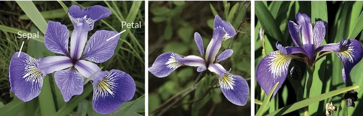
In this case study, we will use the Iris dataset, which contains measurements of sepal length, sepal width, petal length, and petal width for different species of iris flowers. PCA will help reduce the number of dimensions while retaining the most important information about the data. You can get the csv version of this dataset from here.

It has 4 features, Sepal Length, Sepal Width, Petal Length, Petal Width all given in centimeters. In total it has 150 rows of data comprising of 3 species with 50 row for each species. Then a column with its species is also given.

6.5.1 Problem Statement

The goal is to apply PCA to the Iris dataset, which consists of 150 samples with 4 features each. We will:

1. Apply PCA to reduce the dimensionality of the dataset from 4 dimensions to 2 dimensions.
2. Calculate the eigenvalues and eigenvectors of the covariance matrix of the dataset.
3. Use the eigenvalues to determine how much variance is explained by each principal component.
4. Visualize the data and the transformed principal components.

6.5.2 Dataset

The Iris dataset includes the following columns:

Sepal Length	Sepal Width	Petal Length	Petal Width	Species
5.1	3.5	1.4	0.2	Setosa
4.9	3.0	1.4	0.2	Setosa
4.7	3.2	1.3	0.2	Setosa
…	…	…	…	…
6.7	3.0	5.2	2.3	Virginica
6.3	2.5	5.0	1.9	Virginica
6.5	3.0	5.5	2.1	Virginica

6.5.3 Step 1: Data Preparation

First, we will load the Iris dataset and normalize it so that each feature has a mean of 0 and a standard deviation of 1. This normalization step is necessary to ensure that all features contribute equally to the PCA process.

# Load necessary libraries
library(tidyverse)
library(caret)
library(ggplot2)
library(knitr)

# Load the Iris dataset
data(iris)

# Step 1: Normalize the dataset (excluding the Species column)
iris_data <- iris[, 1:4]
iris_data_scaled <- scale(iris_data)

# Check the first few rows of the scaled data
kable(head(iris_data_scaled))

Sepal.Length	Sepal.Width	Petal.Length	Petal.Width
-0.8976739	1.0156020	-1.335752	-1.311052
-1.1392005	-0.1315388	-1.335752	-1.311052
-1.3807271	0.3273175	-1.392399	-1.311052
-1.5014904	0.0978893	-1.279104	-1.311052
-1.0184372	1.2450302	-1.335752	-1.311052
-0.5353840	1.9333146	-1.165809	-1.048667

6.5.4 Step 2: Compute the Covariance Matrix

Next, we will compute the covariance matrix of the normalized dataset. The covariance matrix helps us understand the relationships between the features.

# Step 2: Compute the covariance matrix
cov_matrix <- cov(iris_data_scaled)

# Print the covariance matrix
cov_matrix

             Sepal.Length Sepal.Width Petal.Length Petal.Width
Sepal.Length    1.0000000  -0.1175698    0.8717538   0.8179411
Sepal.Width    -0.1175698   1.0000000   -0.4284401  -0.3661259
Petal.Length    0.8717538  -0.4284401    1.0000000   0.9628654
Petal.Width     0.8179411  -0.3661259    0.9628654   1.0000000

6.5.5 Step 3: Calculate Eigenvalues and Eigenvectors

We will calculate the eigenvalues and eigenvectors of the covariance matrix. The eigenvalues represent the amount of variance explained by each principal component, and the eigenvectors represent the directions of maximum variance.

# Step 3: Calculate the eigenvalues and eigenvectors
eigen_decomp <- eigen(cov_matrix)

# Eigenvalues
eigenvalues <- eigen_decomp$values
print("Eigenvalues:")

[1] "Eigenvalues:"

eigenvalues

[1] 2.91849782 0.91403047 0.14675688 0.02071484

# Eigenvectors
eigenvectors <- eigen_decomp$vectors
print("Eigenvectors:")

[1] "Eigenvectors:"

eigenvectors

           [,1]        [,2]       [,3]       [,4]
[1,]  0.5210659 -0.37741762  0.7195664  0.2612863
[2,] -0.2693474 -0.92329566 -0.2443818 -0.1235096
[3,]  0.5804131 -0.02449161 -0.1421264 -0.8014492
[4,]  0.5648565 -0.06694199 -0.6342727  0.5235971

6.5.6 Step 4: Transform the Data

Using the eigenvectors, we will transform the original data into a new space defined by the principal components.

# Step 4: Transform the data into the new space
# We use the eigenvectors to project the data onto the principal components
pca_data <- iris_data_scaled %*% eigenvectors

# Step 5: Create a DataFrame with the transformed data (first two principal components)
pca_df <- as.data.frame(pca_data[, 1:2])  # Select first two principal components
colnames(pca_df) <- c("PC1", "PC2")
pca_df$Species <- iris$Species

# Check the transformed data
head(pca_df)

        PC1        PC2 Species
1 -2.257141 -0.4784238  setosa
2 -2.074013  0.6718827  setosa
3 -2.356335  0.3407664  setosa
4 -2.291707  0.5953999  setosa
5 -2.381863 -0.6446757  setosa
6 -2.068701 -1.4842053  setosa

6.5.7 Step 5: Visualize the PCA Result

We will use ggplot2 to create a scatter plot of the transformed data in the 2D space defined by the first two principal components.

# Load necessary libraries
library(plotly)
library(datasets)

# Load the Iris dataset
data(iris)

# Perform PCA on the Iris dataset (using prcomp)
pca_result <- prcomp(iris[, 1:4], center = TRUE, scale. = TRUE)

# Create a data frame for the PCA results
pca_df <- as.data.frame(pca_result$x)

# Add the Species column to the PCA results
pca_df$Species <- iris$Species

# Create a 3D scatter plot using plotly
fig <- plot_ly(data = pca_df, 
               x = ~PC1, y = ~PC2, z = ~PC3, 
               color = ~Species, 
               colors = c('red', 'green', 'blue'),
               type = 'scatter3d', mode = 'markers',
               marker = list(size = 5)) %>%
  layout(title = "3D PCA of Iris Dataset",
         scene = list(
           xaxis = list(title = 'Principal Component 1'),
           yaxis = list(title = 'Principal Component 2'),
           zaxis = list(title = 'Principal Component 3')
         ))

# Show the plot
fig