2 Package ggplot2
An elegant modern graphic method based on Wilkinson's Grammar of Graphics
2.1 Maps:
2.1.1 Polygon
library(ggplot2)
require(maps)
## Loading required package: mapsportugal = map_data('world', region = 'Portugal')
ggplot(portugal, aes(x = long, y = lat, group = group)) +
geom_polygon(fill = 'white', colour = 'black')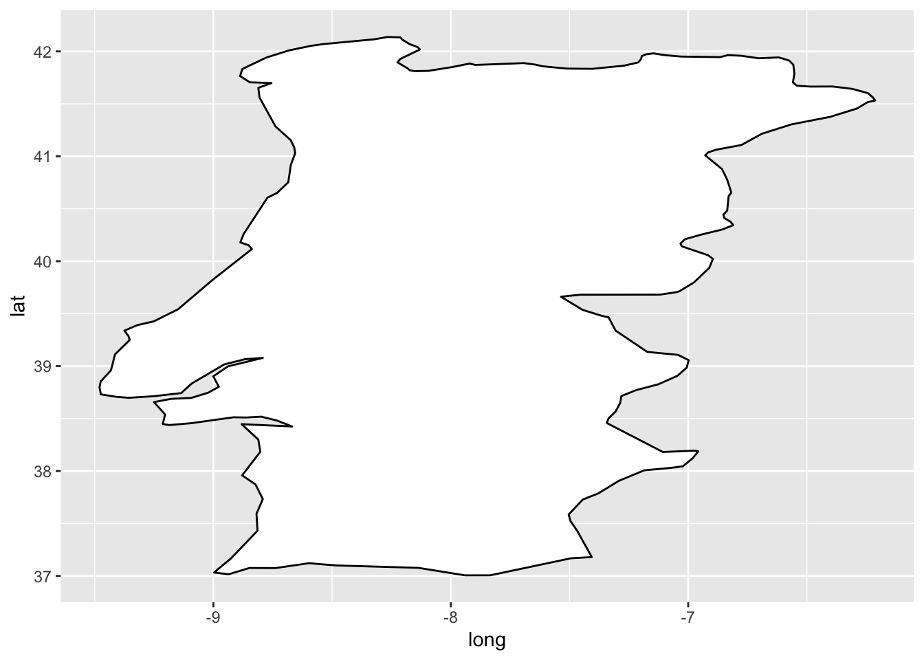
2.2 Path, ribbon and rectangles.
h <- ggplot(economics, aes(date, unemploy))
# Path
h + geom_path() 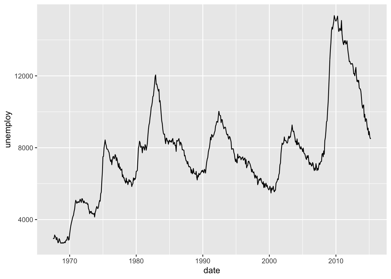
# Ribbon
h + geom_ribbon(aes(ymin = unemploy-900, ymax = unemploy+900), fill = "steelblue") + geom_path(size = 0.8) 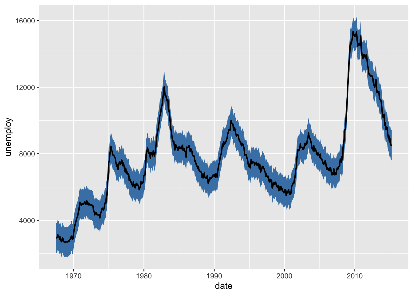
# Rectangle
h + geom_rect(aes(xmin = as.Date('1980-01-01'), ymin = -Inf, xmax = as.Date('1985-01-01'), ymax = Inf), fill = "steelblue") + geom_path(size = 0.8) 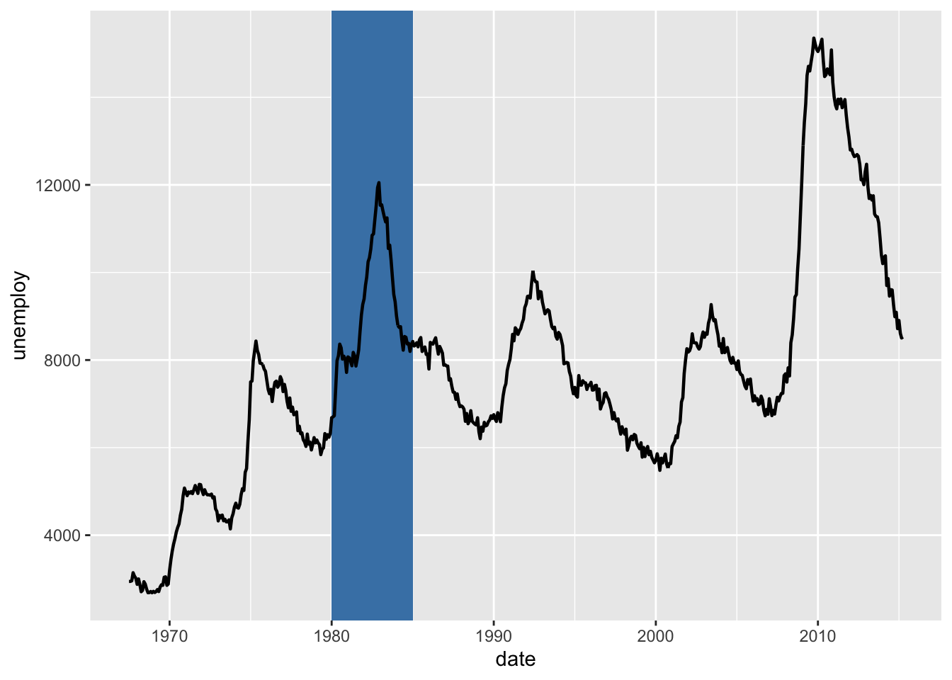
2.2.1 Add line segments between points (x1, y1) and (x2, y2):
2.2.1.1 Create a scatter plot
i <- ggplot(mtcars, aes(wt, mpg)) + geom_point()
# Add segment
i + geom_segment(aes(x = 2, y = 15, xend = 3, yend = 15)) 
# Add arrow require(grid)
i + geom_segment(aes(x = 5, y = 30, xend = 3.5, yend = 25), arrow = arrow(length = unit(0.5, "cm")))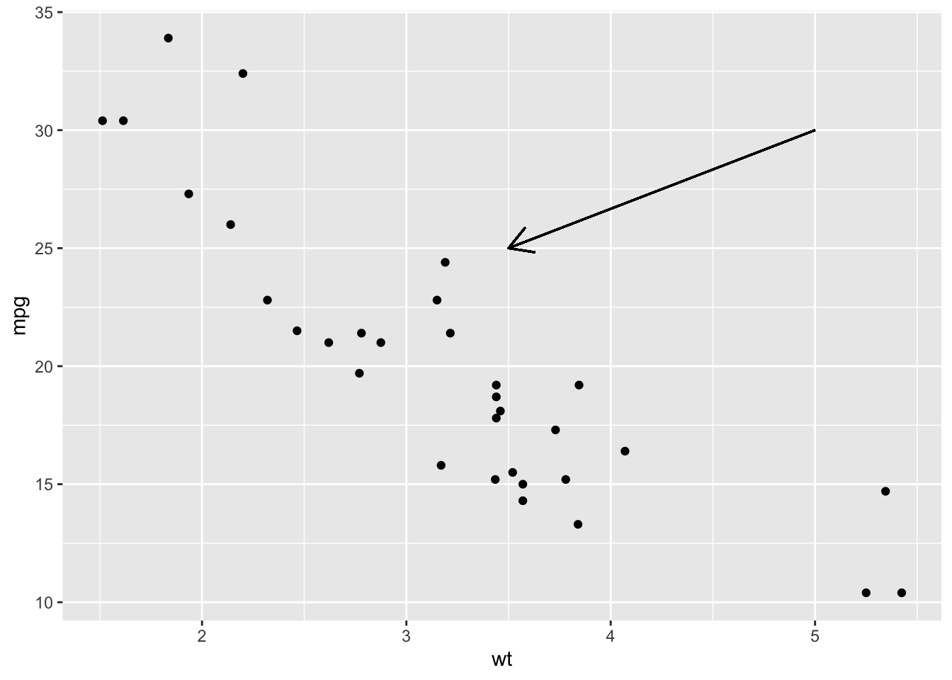
2.2.1.2 Add curves between points (x1, y1) and (x2, y2):
i + geom_curve(aes(x = 2, y = 15, xend = 3, yend = 15))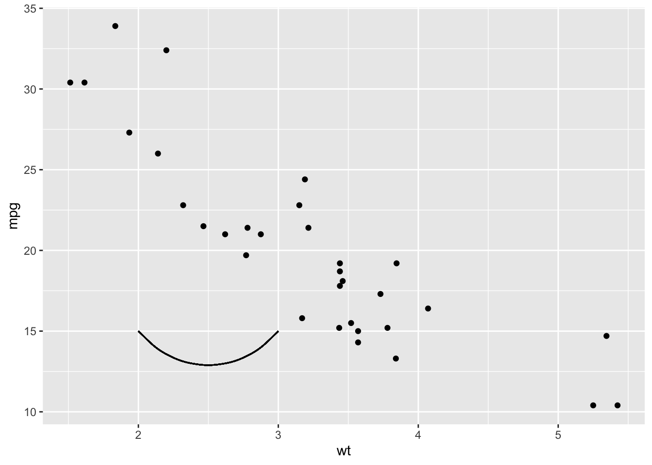
2.3 Graphical parameters:
2.3.1 Convert the variable dose from numeric to factor variable
ToothGrowth$dose <- as.factor(ToothGrowth$dose)
p <- ggplot(ToothGrowth, aes(x=dose, y=len))
p+ geom_boxplot()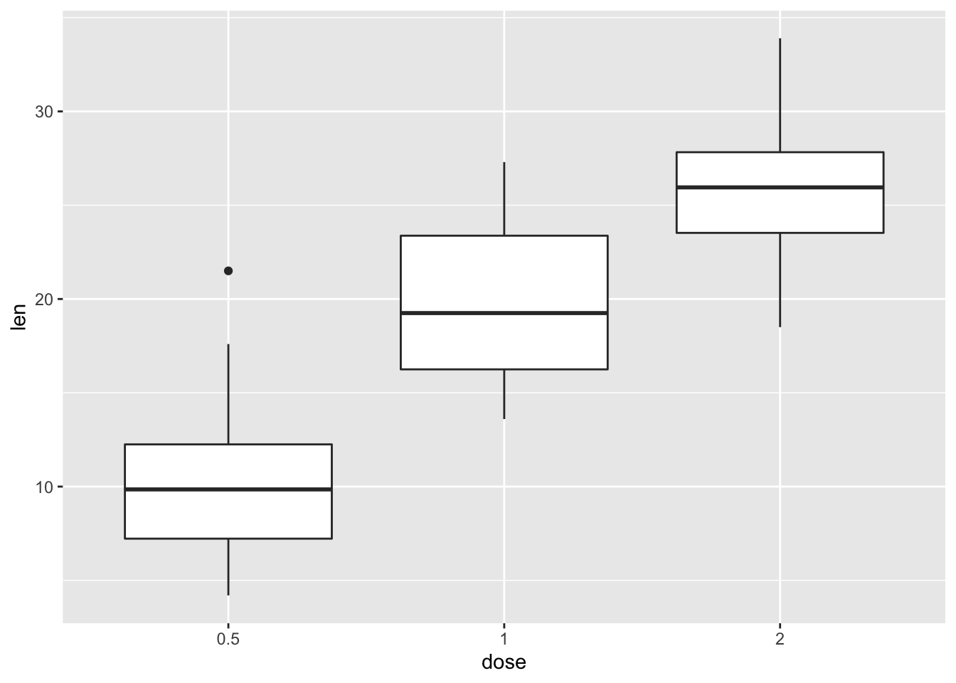
2.3.2 Default plot
print(p) 
2.3.3 Change title and axis labels
p1 <- p +labs(title="Plot of length \n by dose", x ="Dose (mg)", y = "Teeth length")
p1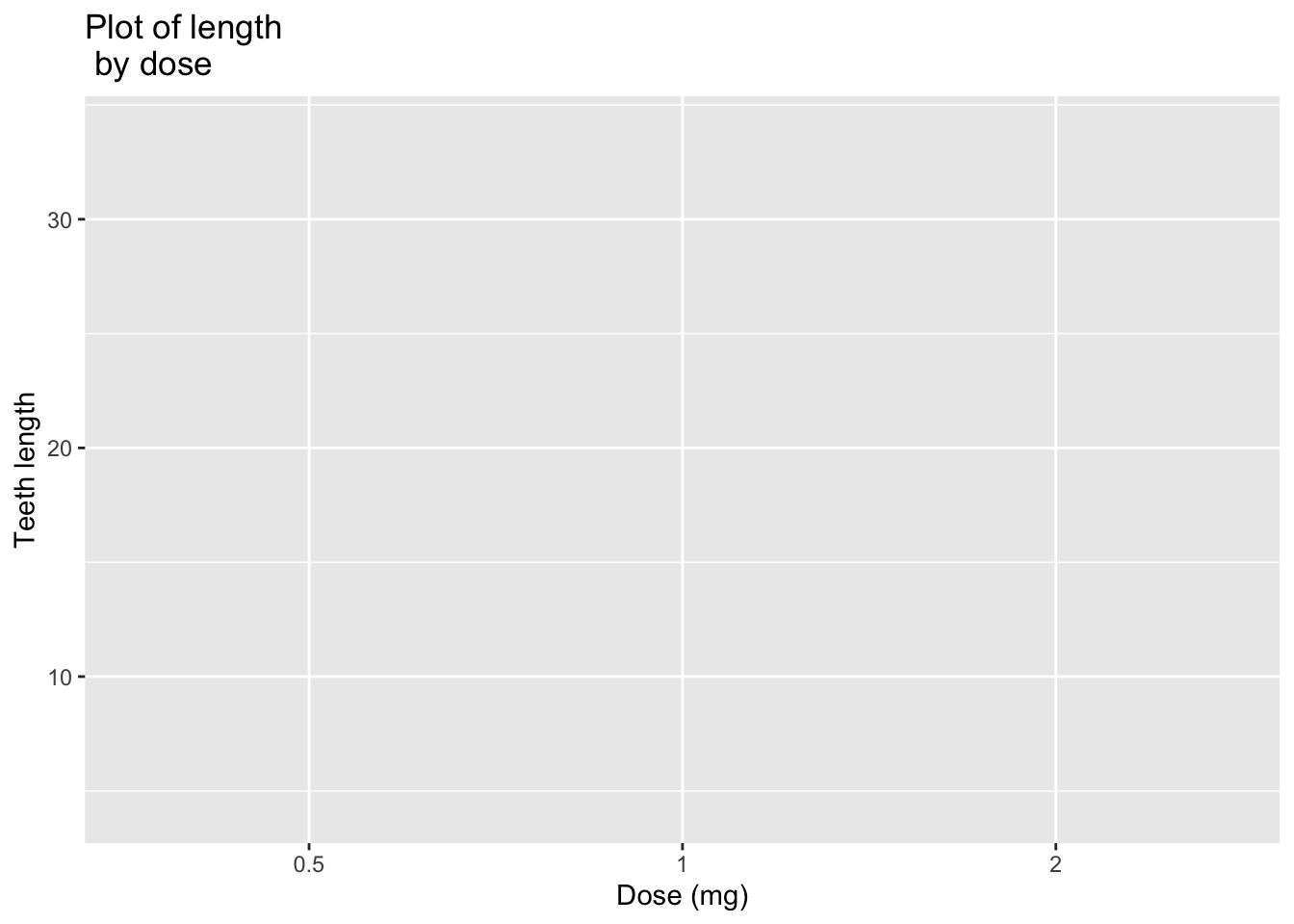
2.3.4 Change the appearance of labels
p1 + theme( plot.title = element_text(color="violet", size=14, face="bold.italic"), axis.title.x = element_text(color="blue", size=14, face="bold"), axis.title.y = element_text(color="blue", size=14, face="bold") ) 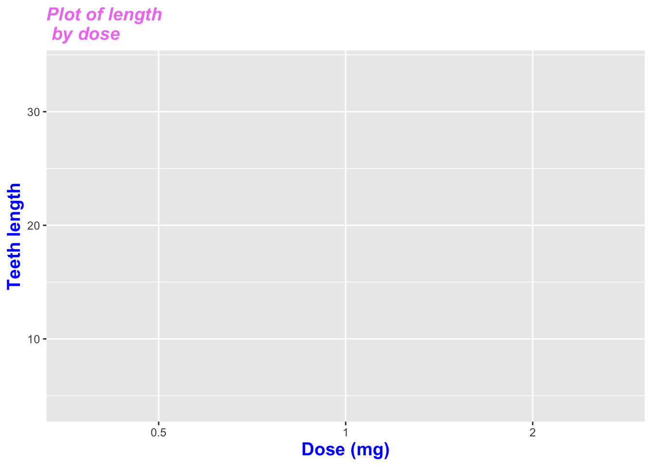
# Hide labels
p1 + theme(plot.title = element_blank(), axis.title.x = element_blank(), axis.title.y = element_blank())
2.3.5 Default plot
p <- ggplot(ToothGrowth, aes(x=dose, y=len, fill=dose))+ geom_boxplot()
p 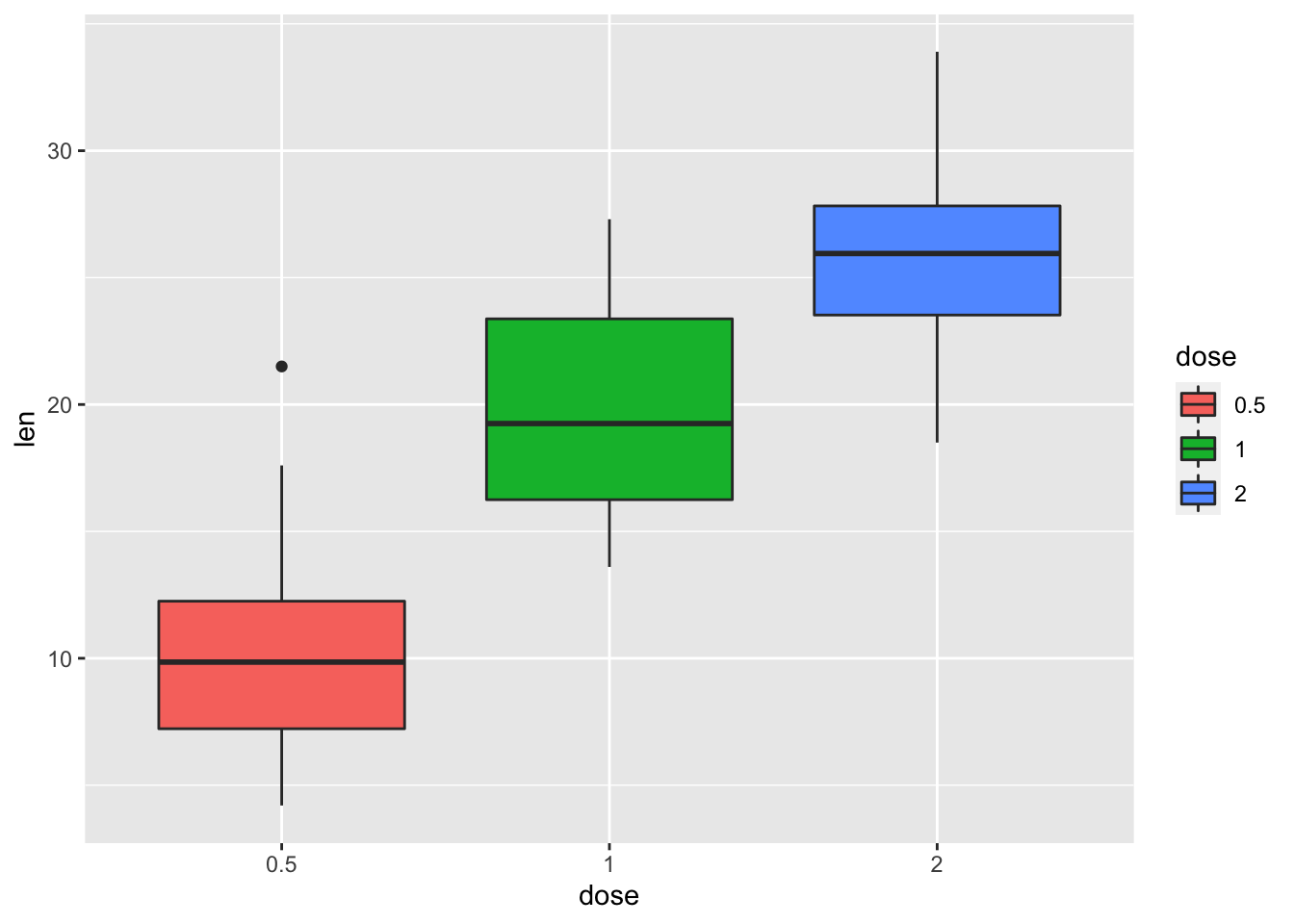
# Modify legend titles
p + labs(fill = "Dose (mg)")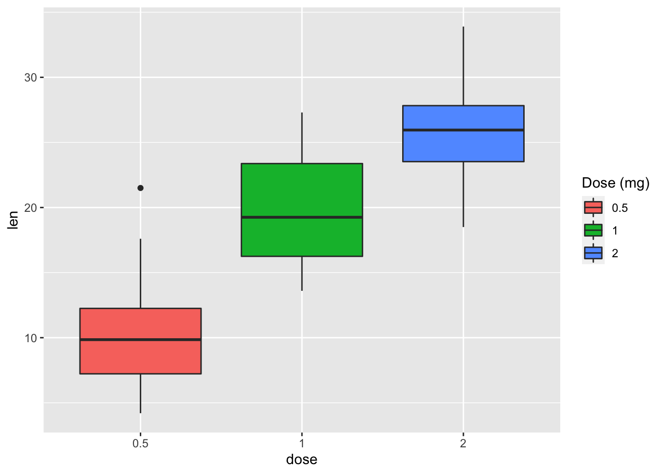
2.4 Legend position and appearance
2.4.1 Convert the variable dose from numeric to factor variable
ToothGrowth$dose <- as.factor(ToothGrowth$dose)
p <- ggplot(ToothGrowth, aes(x=dose, y=len, fill=dose))+
      geom_boxplot()
2.4.2 Change legend position: "left","top", "right", "bottom", "none"
p + theme(legend.position="top") 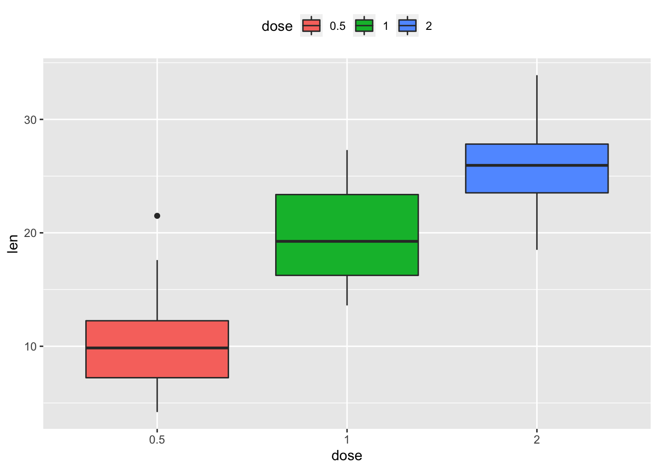
2.4.3 Remove legends
p + theme(legend.position = "none") 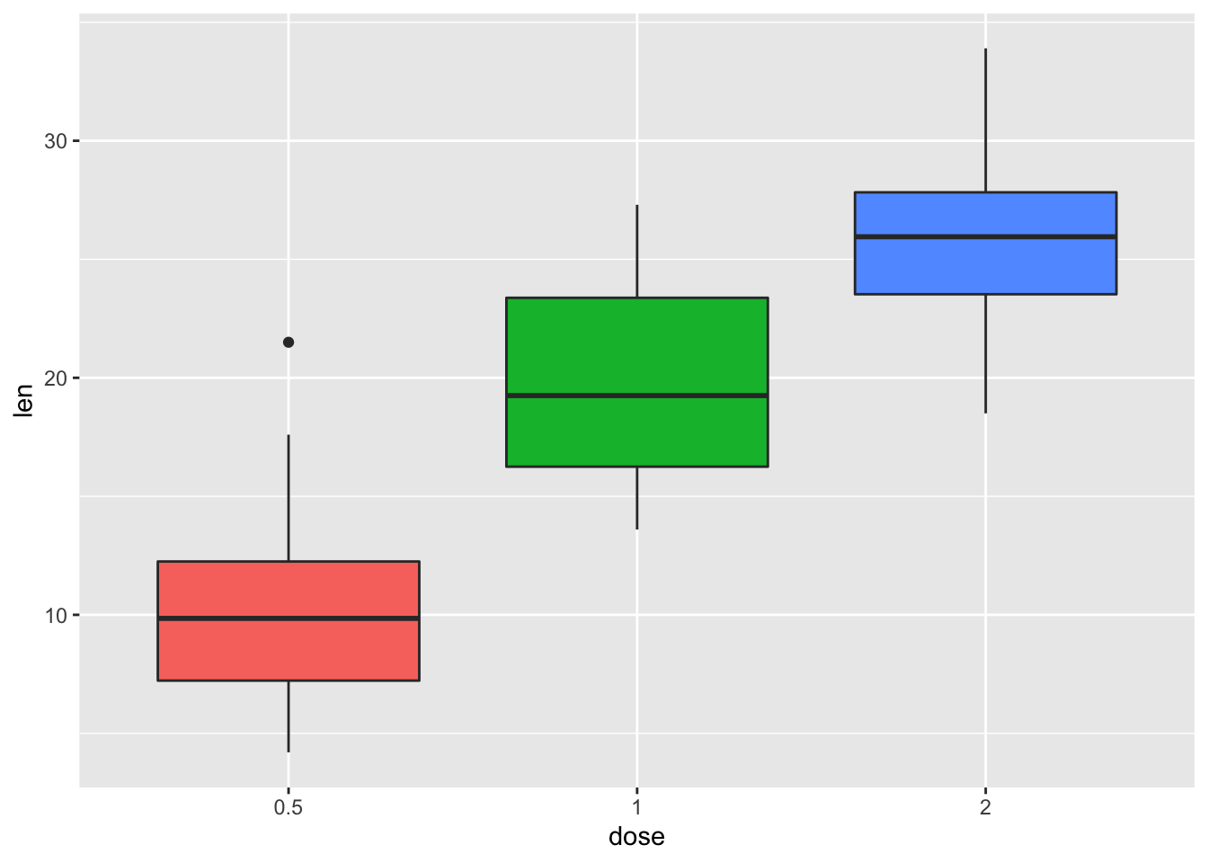
# Change the appearance of legend title and labels
p + theme(legend.title = element_text(colour="darkgreen"), legend.text = element_text(colour="red")) 
# Change legend box background color
p + theme(legend.background = element_rect(fill="violet"))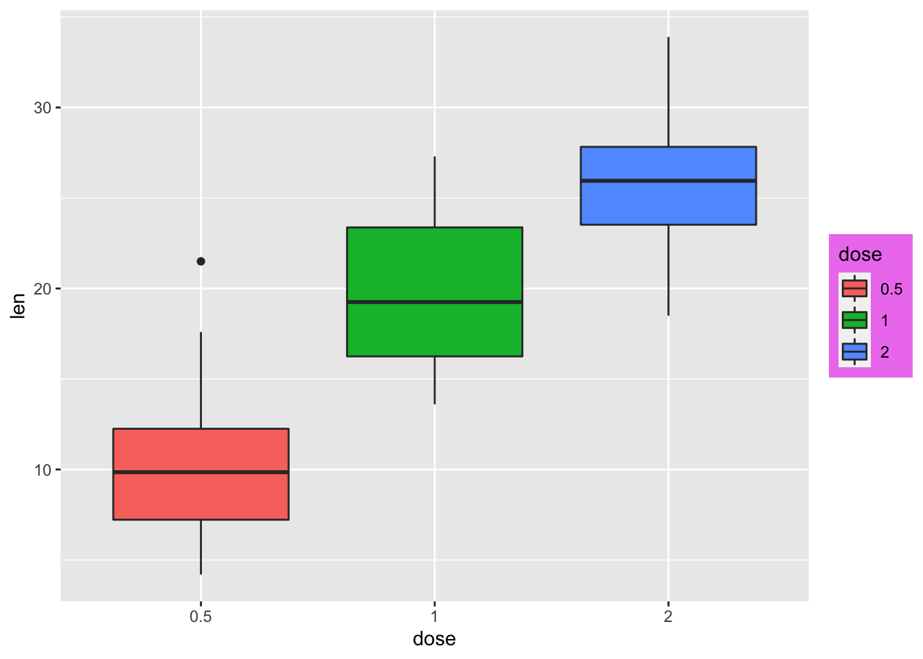
2.4.4 Change the order of legend items
p + scale_x_discrete(limits=c("2", "0.5", "1"))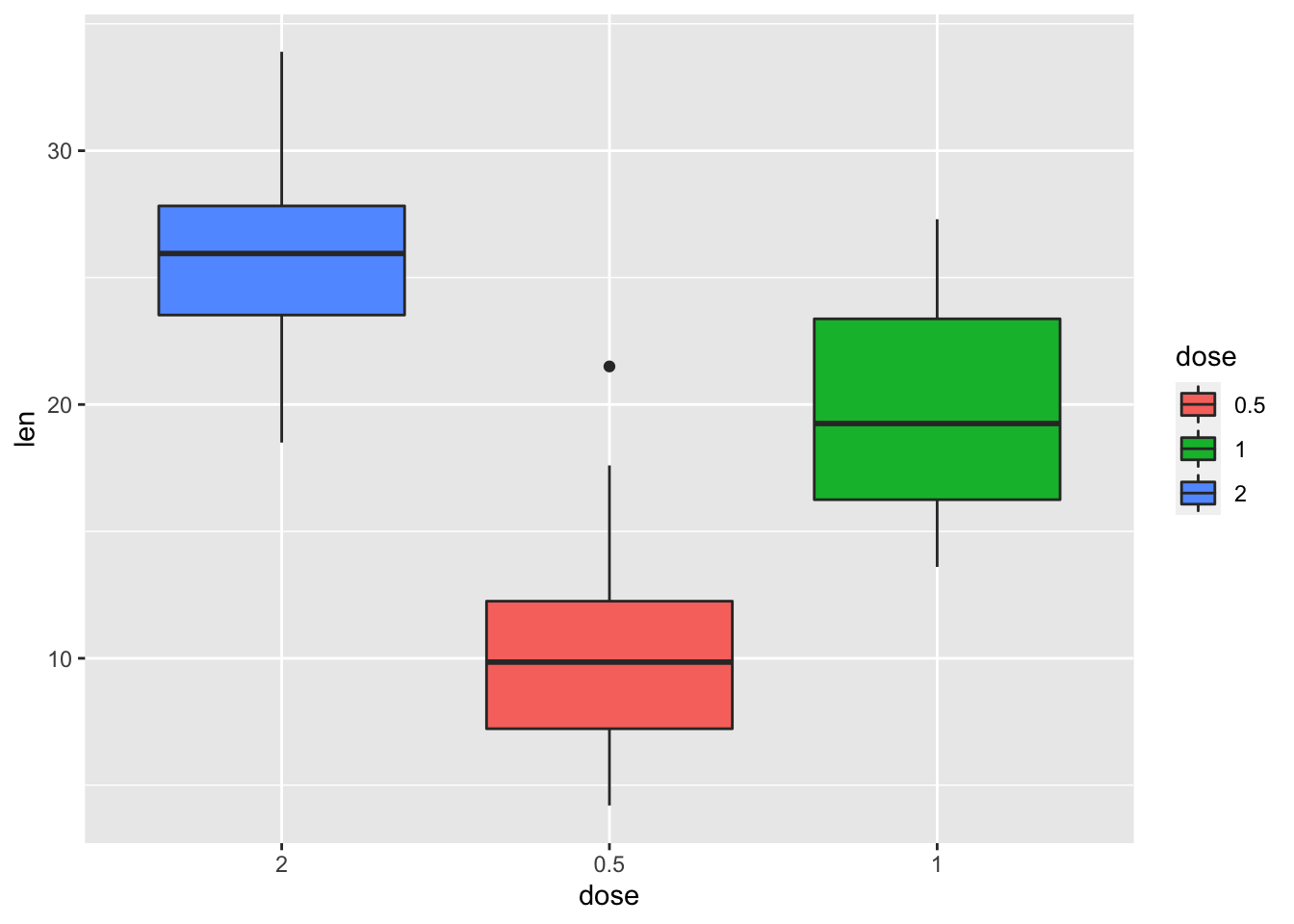
# Set legend title and labels
p + scale_fill_discrete(name = "Dose", labels = c("A", "B", "C"))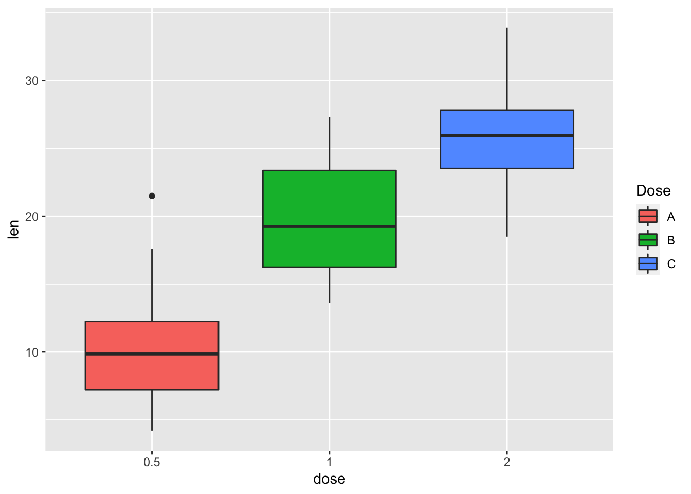
2.4.5 Convert dose and cyl columns from numeric to factor variables
ToothGrowth$dose <- as.factor(ToothGrowth$dose)
mtcars$cyl <- as.factor(mtcars$cyl)
2.4.6 Box plot and scatterplot
bp <- ggplot(ToothGrowth, aes(x=dose, y=len))
# Scatter plot
sp <- ggplot(mtcars, aes(x=wt, y=mpg))
bp + geom_boxplot(fill='steelblue', color="violet") 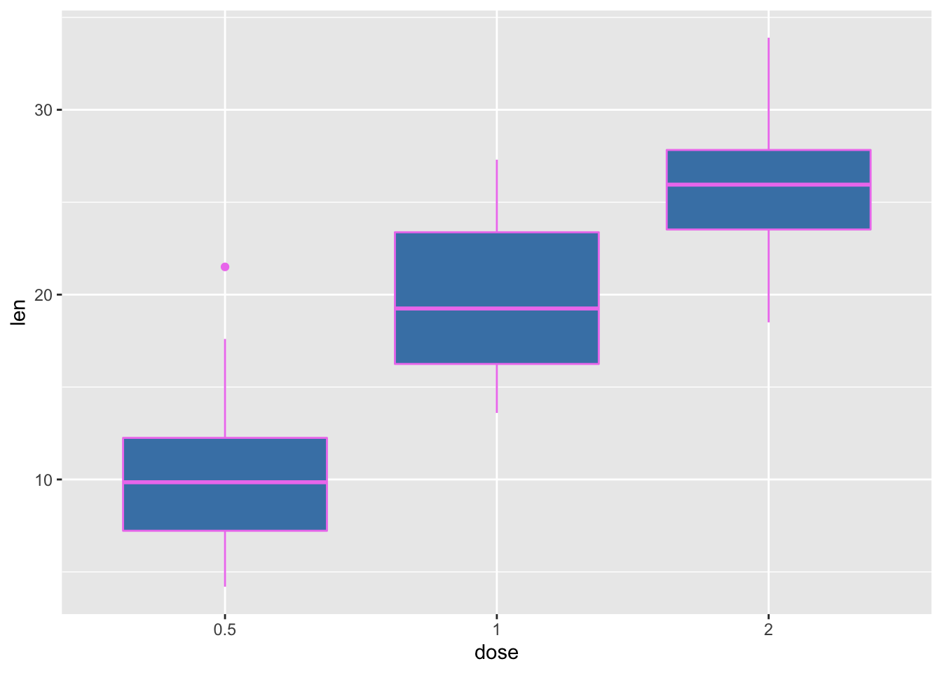
# scatter plot
sp + geom_point(color='darkblue')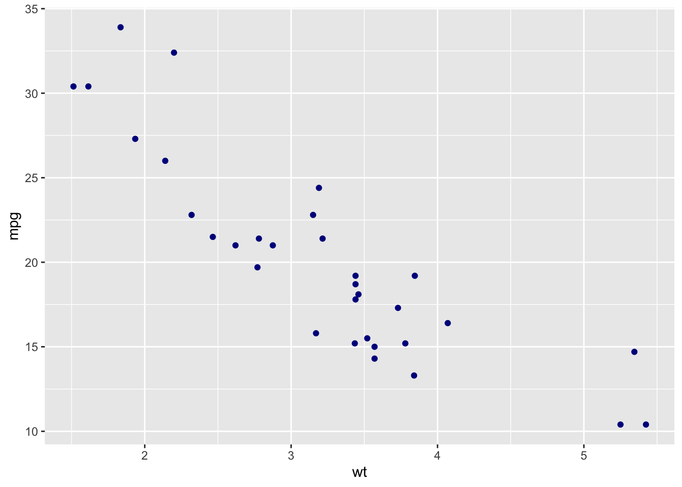
2.4.7 Box plot
bp <- bp + geom_boxplot(aes(fill = dose))
bp 
2.4.8 Scatter plot
sp <- sp + geom_point(aes(color = cyl))
sp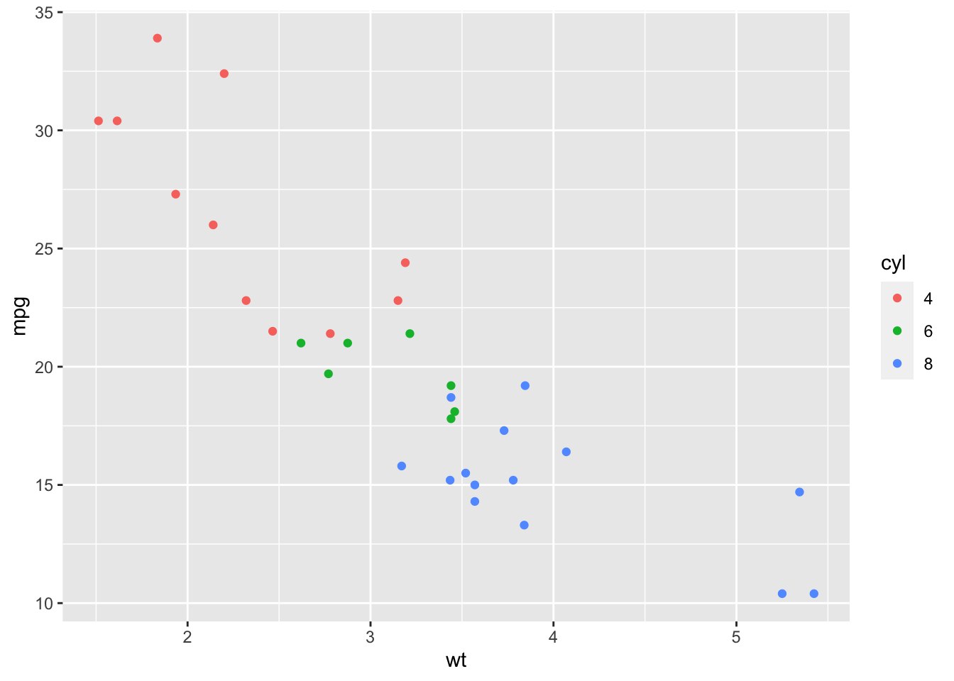
2.5 Color by qsec values
sp2<-ggplot(mtcars, aes(x=wt, y=mpg)) + geom_point(aes(color = qsec))
sp2 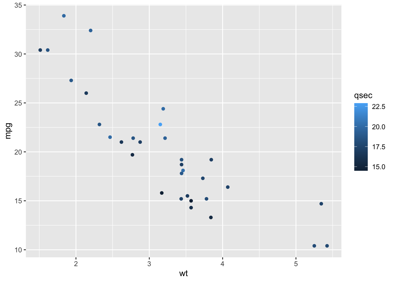
2.6 Change the low and high colors Sequential color scheme
sp2+scale_color_gradient(low="blue", high="red") 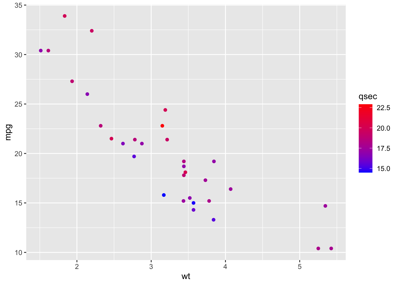
2.7 Diverging color scheme
mid<-mean(mtcars$qsec)
sp2+scale_color_gradient2(midpoint=mid, low="blue", mid="white", high="red", space = "Lab" )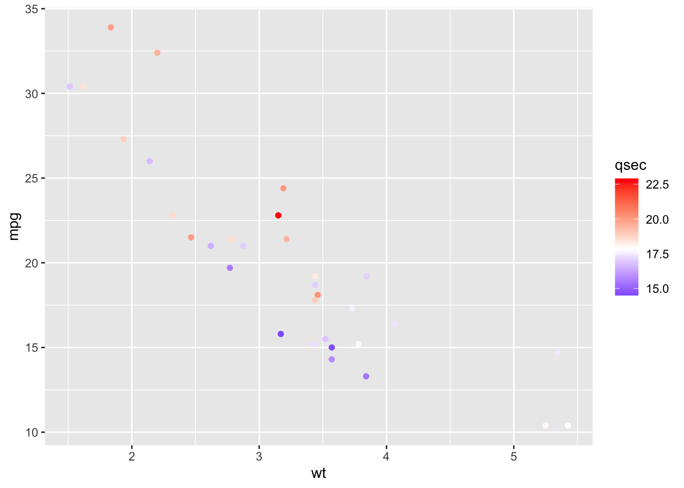
2.8 Point shapes, colors and size
knitr::include_graphics("shapes.png")
2.9 Convert cyl as factor variable
mtcars$cyl <- as.factor(mtcars$cyl)2.9.1 Basic scatter plot
ggplot(mtcars, aes(x=wt, y=mpg)) +
geom_point(shape = 18, color = "steelblue", size = 4) 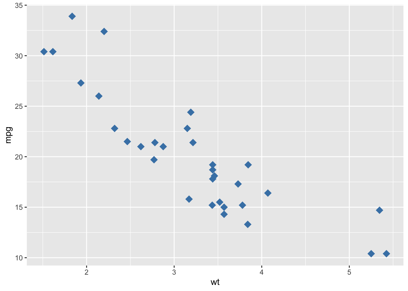
2.9.2 Change point shapes and colors by groups
ggplot(mtcars, aes(x=wt, y=mpg)) +
      geom_point(aes(shape = cyl, color = cyl))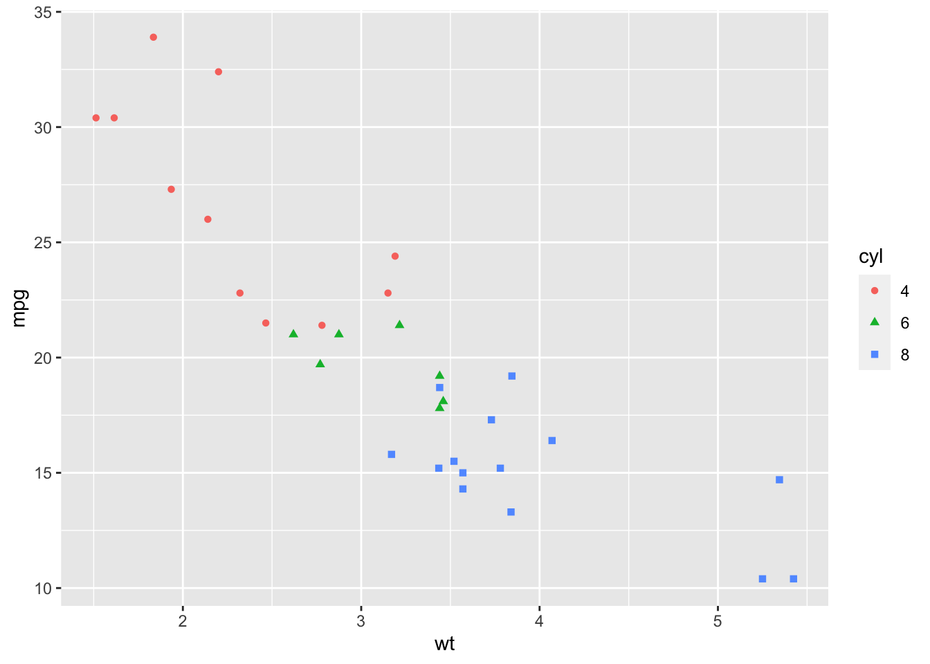
2.9.3 Change colors and shapes manually
ggplot(mtcars, aes(x=wt, y=mpg, group=cyl)) + geom_point(aes(shape=cyl, color=cyl), size=2)+ scale_shape_manual(values=c(3, 16, 17))+ scale_color_manual(values=c('#999999','#E69F00', '#56B4E9'))+ theme(legend.position="top")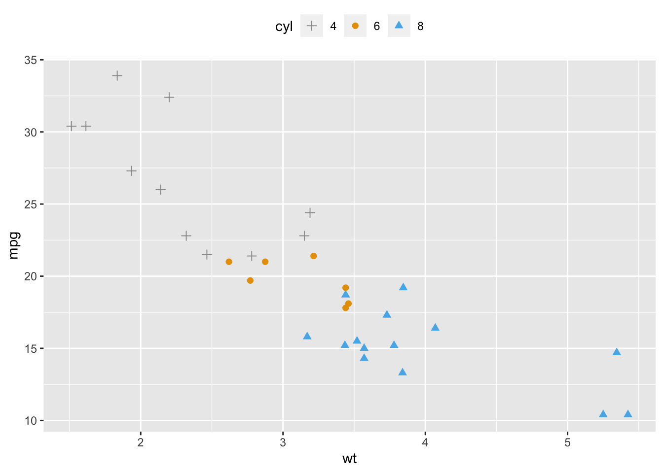
2.9.4 Add text annotations to a graph
set.seed(1234)
df <- mtcars[sample(1:nrow(mtcars), 10), ]
df$cyl <- as.factor(df$cyl)
2.9.5 Line types
knitr::include_graphics("lines.png")
2.10 Basic line plot
2.10.1 Create some data
df <- data.frame(time=c("breakfeast", "Lunch", "Dinner"), bill=c(10, 30, 15))
head(df)
## time bill
## 1 breakfeast 10
## 2 Lunch 30
## 3 Dinner 152.10.2 Basic line plot with points
Change the line type
ggplot(data=df, aes(x=time, y=bill, group=1)) +
      geom_line(linetype = "dashed")+
      geom_point()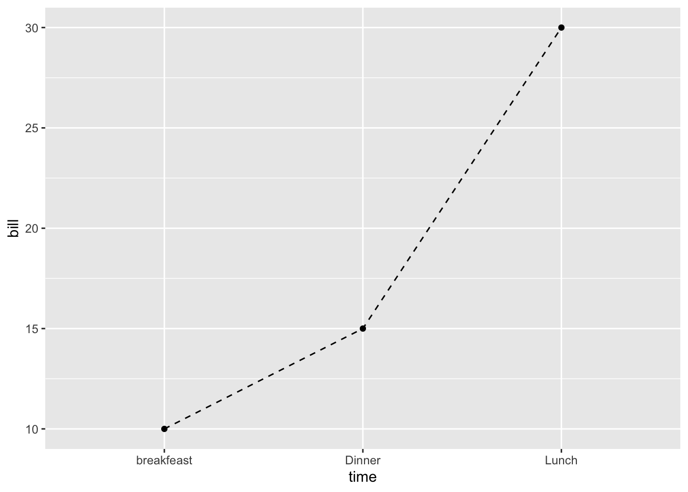
2.11 Line plots with multiple groups
2.11.1 Create some data
df2 <- data.frame(sex = rep(c("Female", "Male"), each=3), time=c("breakfeast", "Lunch", "Dinner"), bill=c(10, 30, 15, 13, 40, 17) )
head(df2, n=3)
## sex time bill
## 1 Female breakfeast 10
## 2 Female Lunch 30
## 3 Female Dinner 152.11.2 Change line types and colors by groups (sex)
ggplot(df2, aes(x=time, y=bill, group=sex)) +
      geom_line(aes(linetype = sex, color = sex))+
      geom_point(aes(color=sex))+
      theme(legend.position="top")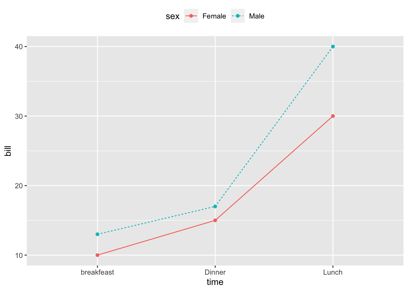
2.12 Change line types, colors and sizes
ggplot(df2, aes(x=time, y=bill, group=sex)) +
      geom_line(aes(linetype=sex, color=sex, size=sex))+ geom_point()+ scale_linetype_manual(values=c("twodash", "dotted"))+ scale_color_manual(values=c('#999999','#E69F00'))+ scale_size_manual(values=c(1, 1.5))+ theme(legend.position="top")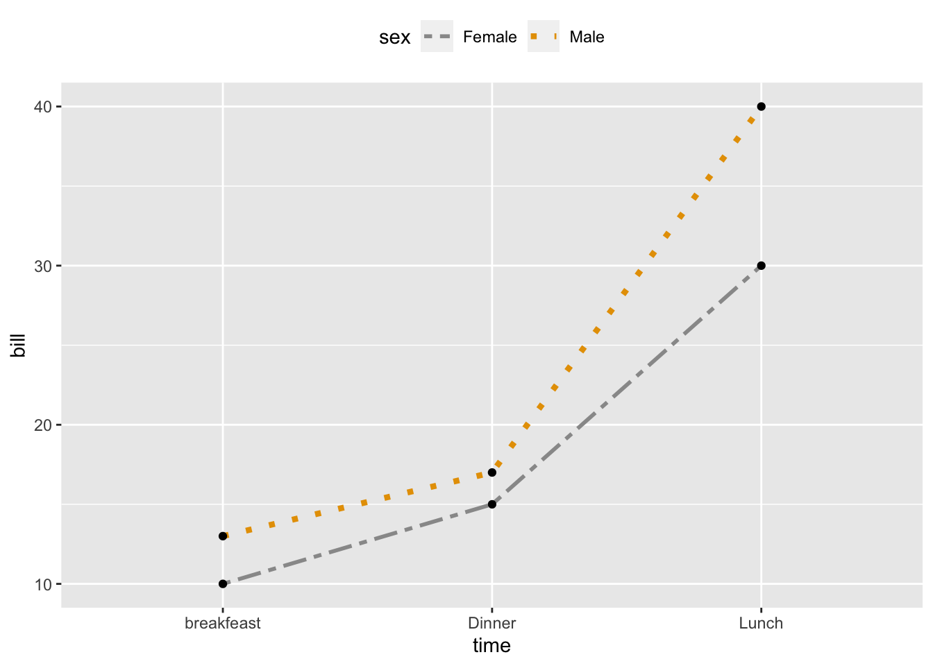
2.13 Themes and background colors
2.13.1 Convert the column dose from numeric to factor variable
ToothGrowth$dose <- as.factor(ToothGrowth$dose)
#Create a box plot
p <- ggplot(ToothGrowth, aes(x=dose, y=len)) +
      geom_boxplot()
2.14 Change plot themes
p + theme_gray(base_size = 14)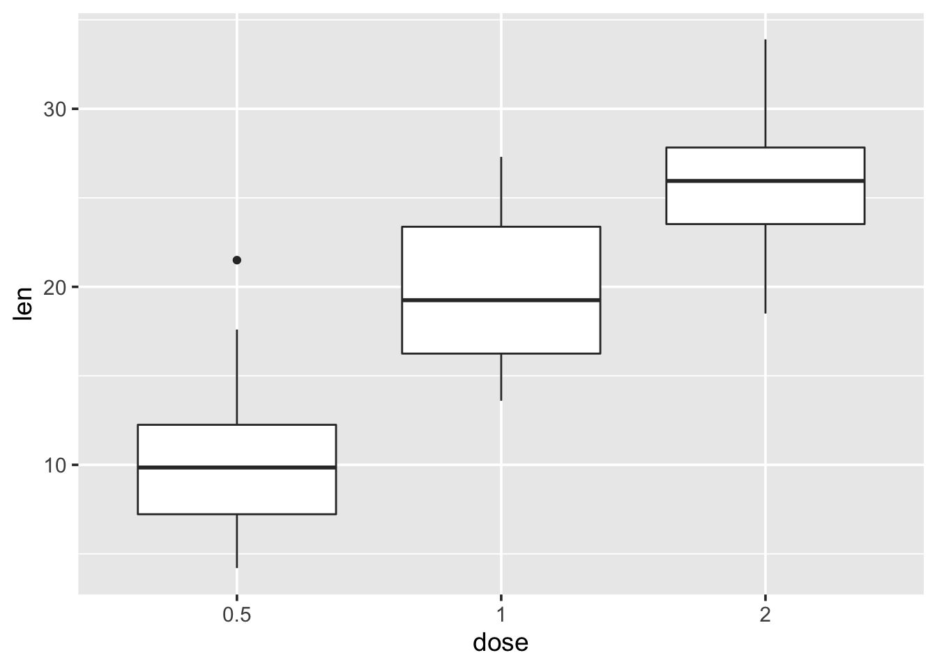
p + theme_bw()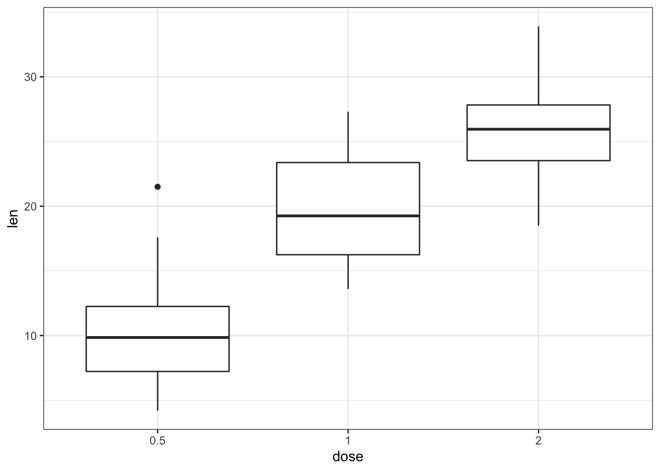
p + theme_linedraw() 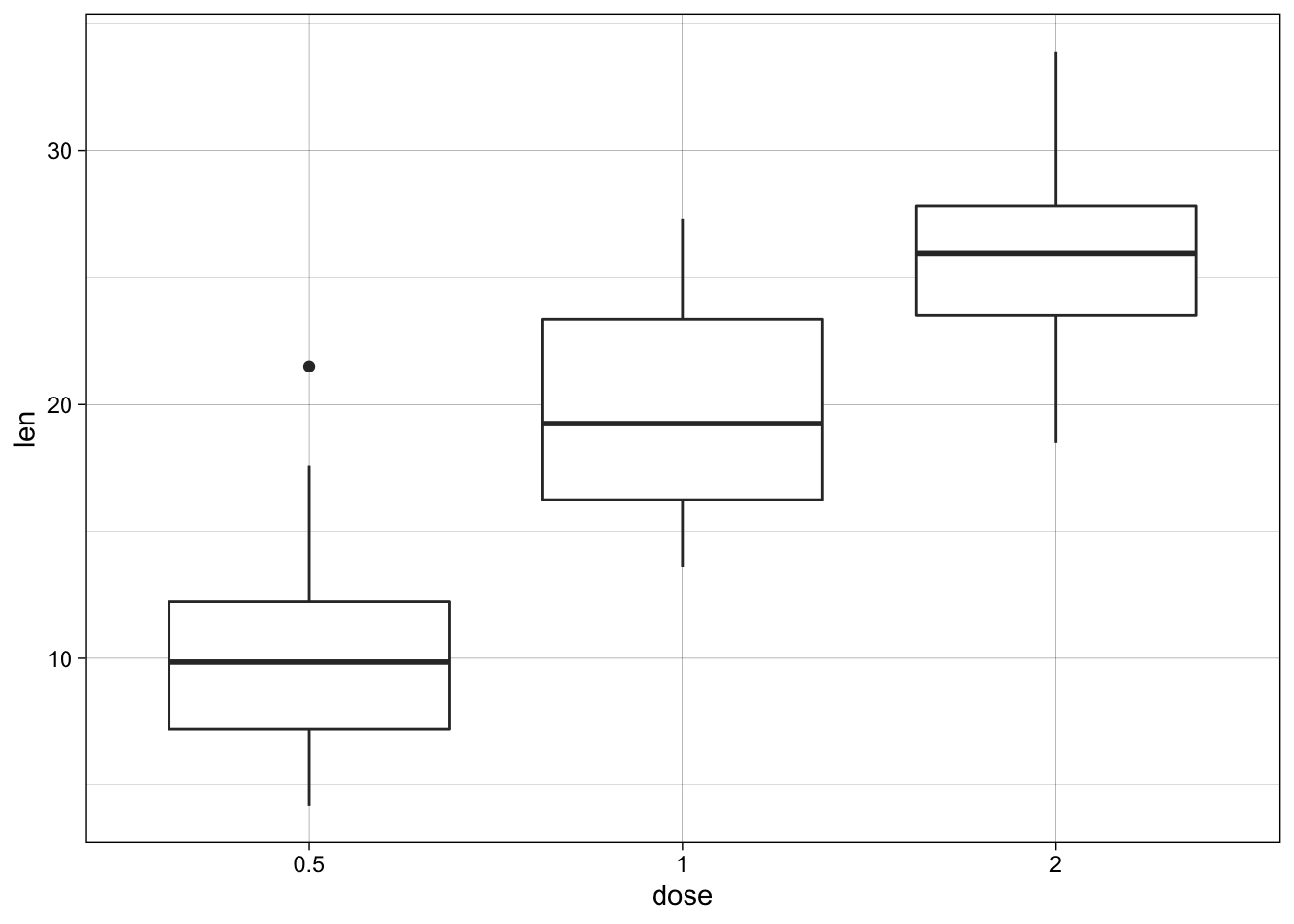
p + theme_light()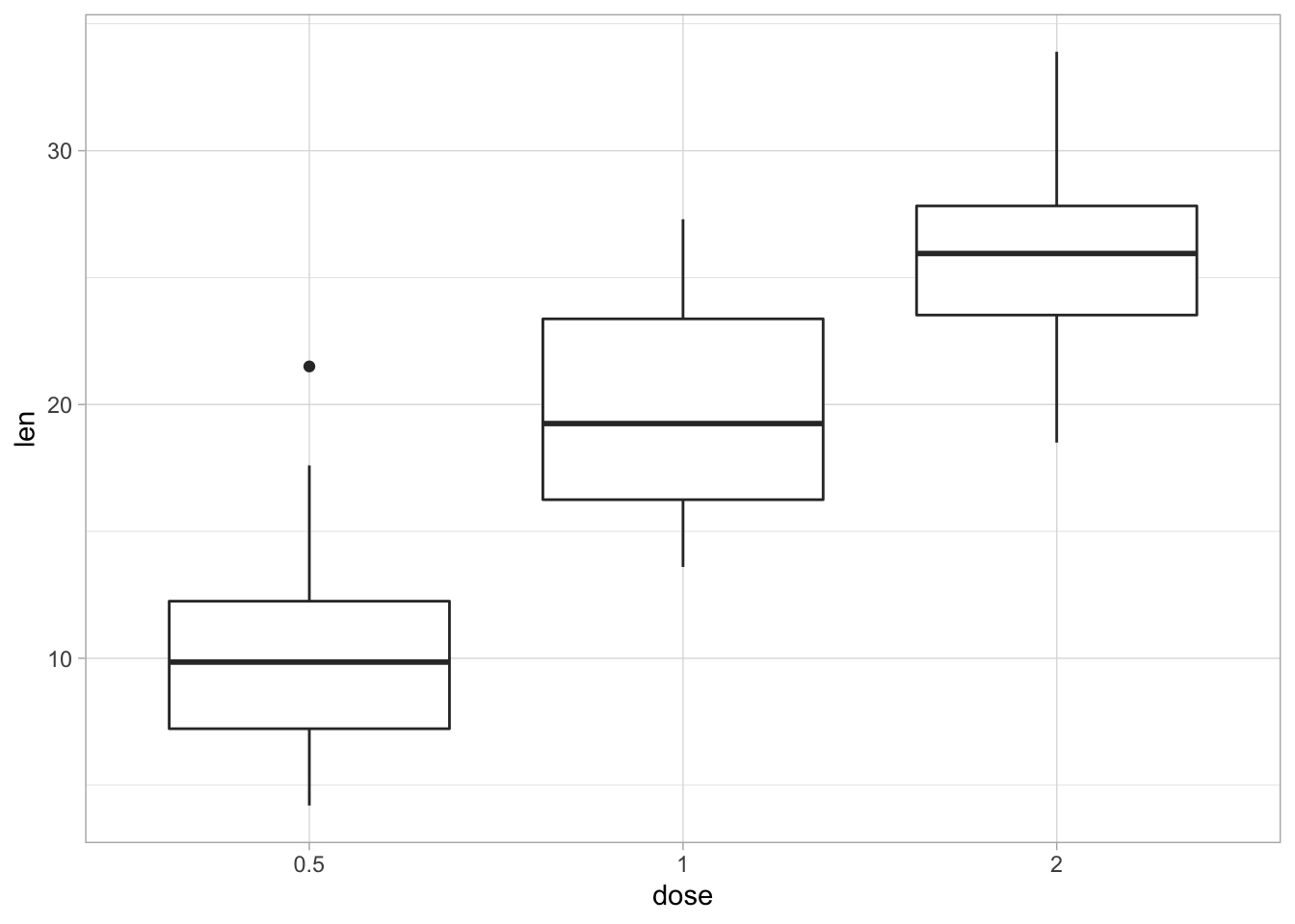
p + theme_minimal() 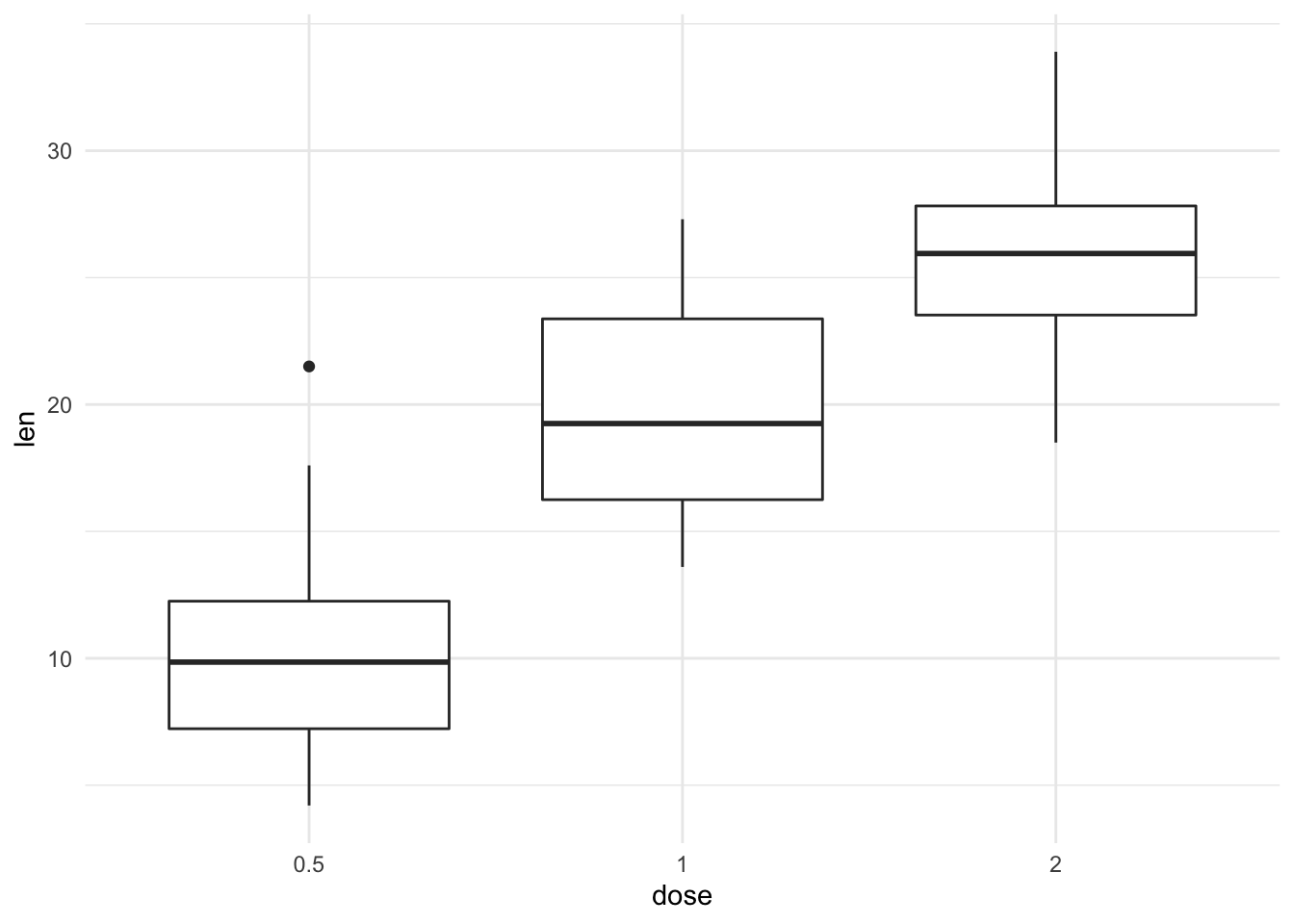
p + theme_classic()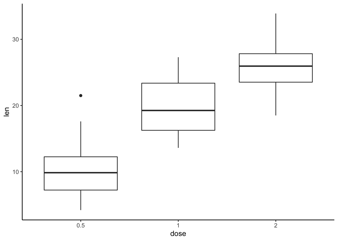
2.15 Axis limits: Minimum and Maximum values
p <- ggplot(cars, aes(x = speed, y = dist)) +
      geom_point()
2.15.1 Different functions are available for setting axis limits:
2.16 Default plot
print(p) ## Change axis limits using coord_cartesian()
p + coord_cartesian(xlim =c(5, 20), ylim = c(0, 50)) 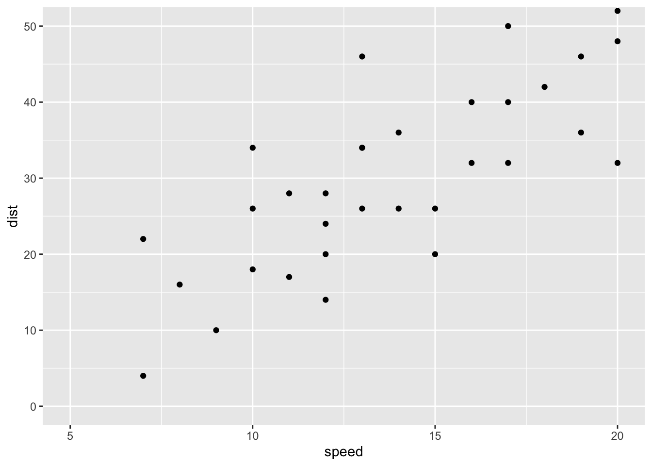
# Use xlim() and ylim()
p + xlim(5, 20) + ylim(0, 50)
## Warning: Removed 19 rows containing missing values (geom_point).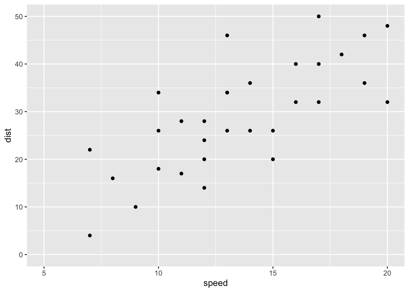
# Expand limits
p + expand_limits(x = c(5, 50), y = c(0, 150))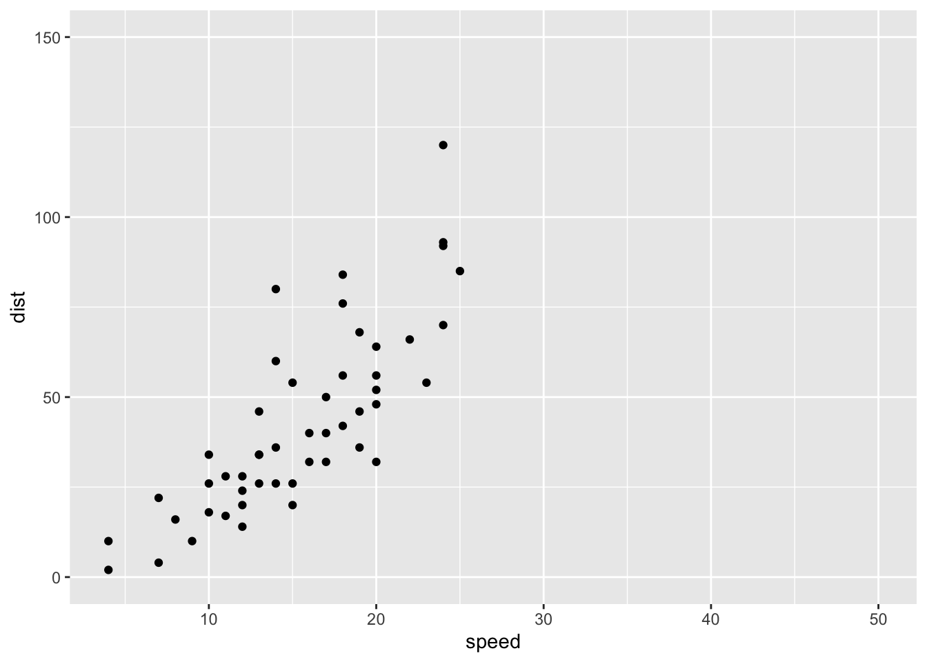
2.17 Axis transformations: log and sqrt scales
2.17.1 Create a scatter plot:
p <- ggplot(cars, aes(x = speed, y = dist)) + geom_point()2.18 Log transformation using scale_xx() # possible values for trans : 'log2', 'log10','sqrt'
p + scale_x_continuous(trans='log2') +
scale_y_continuous(trans='log2') 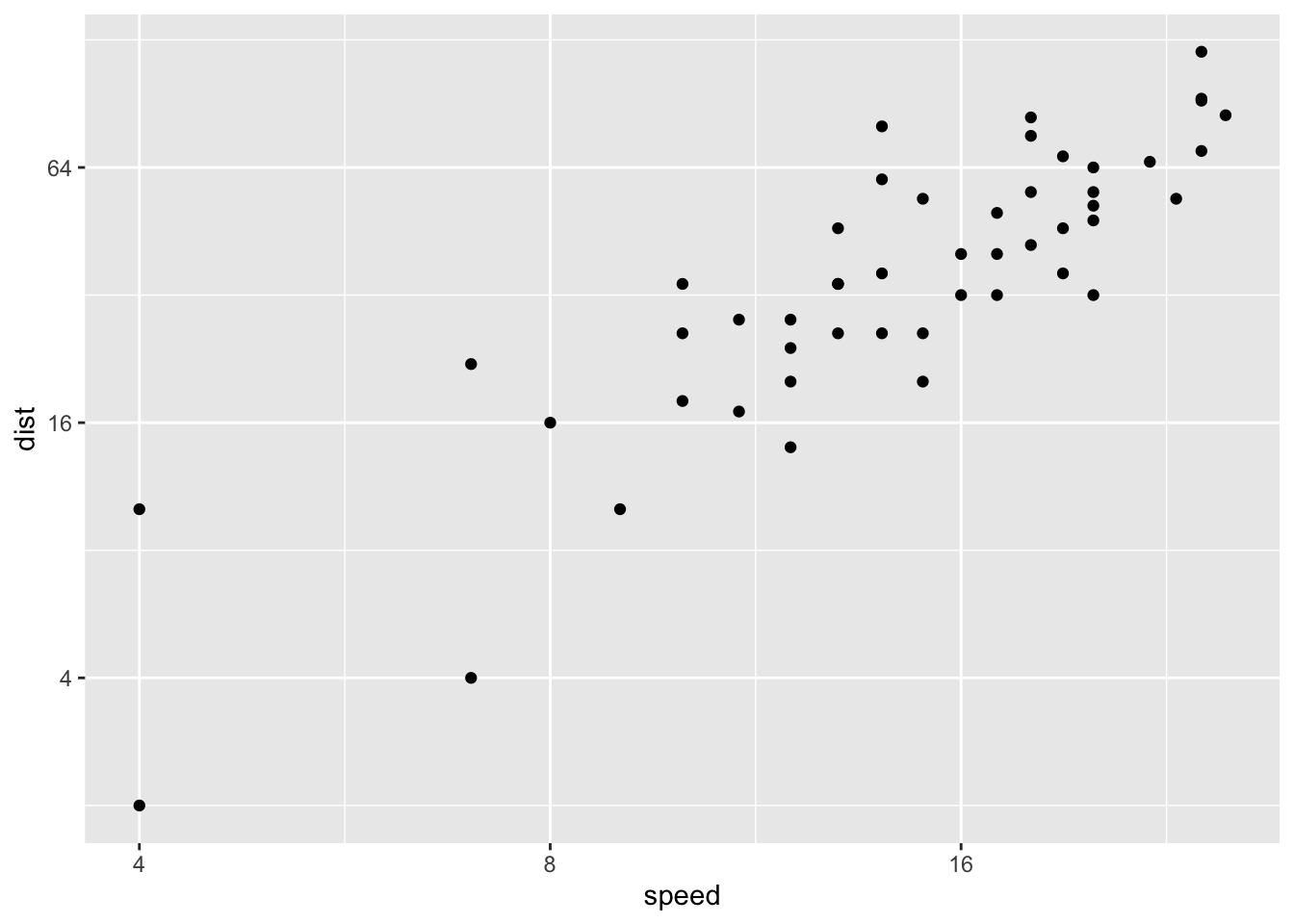
2.19 Format axis tick mark labels
require(scales)## Loading required package: scales##
## Attaching package: 'scales'## The following object is masked from 'package:readr':
##
## col_factorp + scale_y_continuous(trans = log2_trans(), breaks = trans_breaks("log2", function(x) 2^x), labels = trans_format("log2", math_format(2^.x))) 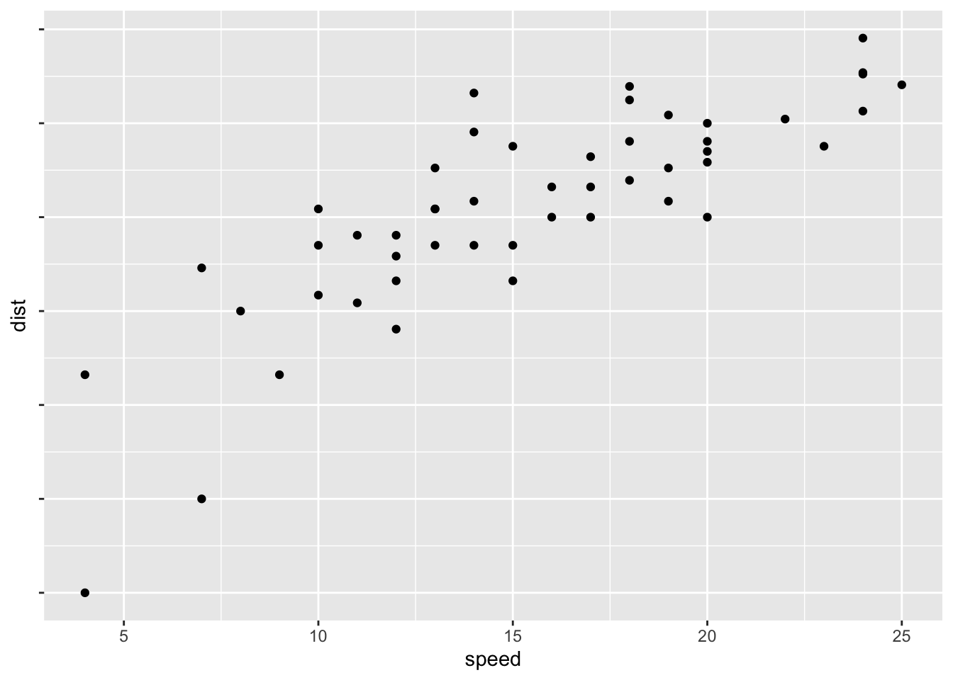
# Reverse coordinates
p + scale_y_reverse() 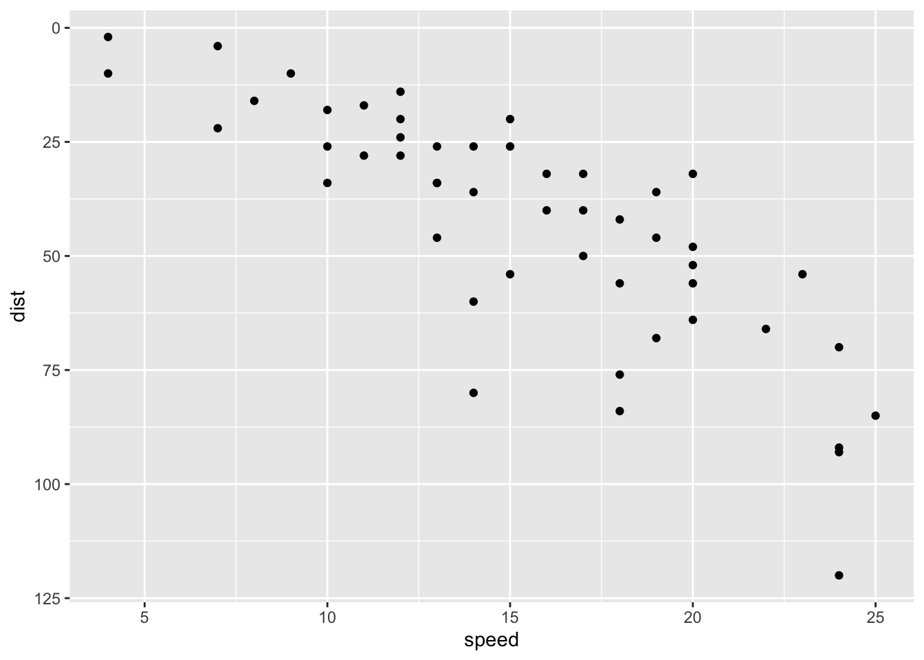
2.20 Axis ticks: customize tick marks and labels, reorder and select items
2.20.1 Create a box plot:
p <- ggplot(ToothGrowth, aes(x=dose, y=len)) + geom_boxplot() 2.21 Change the style and the orientation angle of axis tick labels face can be "plain", "italic", "bold" or "bold.italic"
p + theme(axis.text.x = element_text(face="bold", color="#993333", size=14, angle=45), axis.text.y = element_text(face="bold", color="blue", size=14, angle=45)) 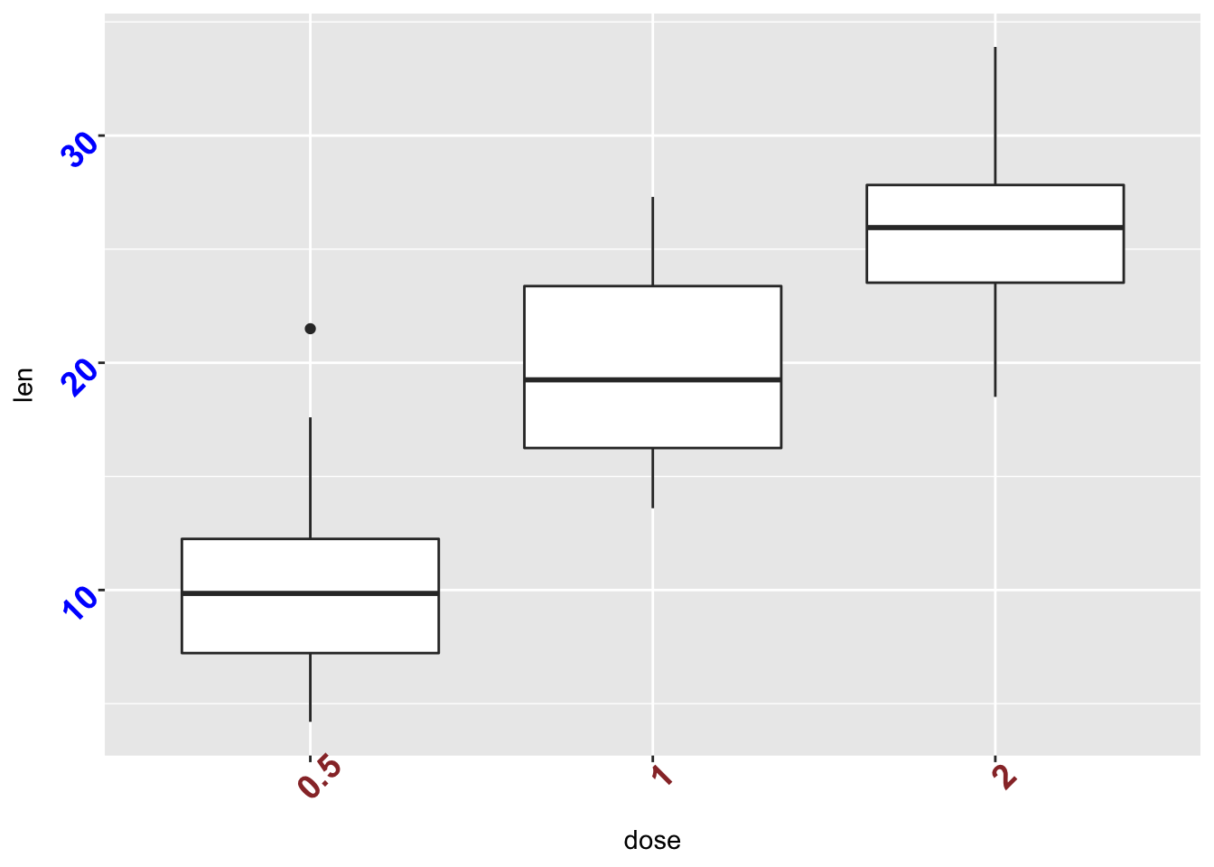
# Remove axis ticks and tick mark labels
p + theme( axis.text.x = element_blank(), # Remove x axis tick labels
axis.text.y = element_blank(), # Remove y axis tick labels
axis.ticks = element_blank()) # Remove ticks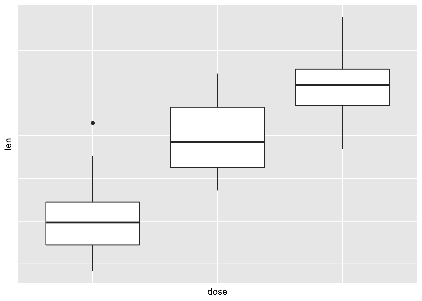 ## Customize continuous and discrete axes: ### Discrete axes:
2.21.1 Change x axis label and the order of items
p + scale_x_discrete(name ="Dose (mg)", limits=c("2","1","0.5")) 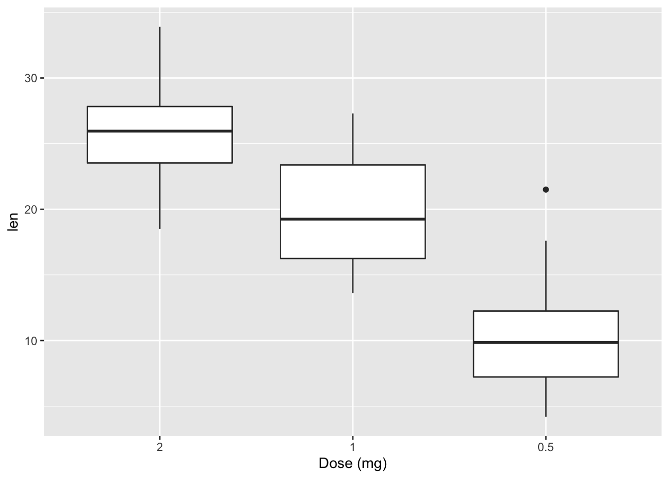
2.21.2 Change tick mark labels
p + scale_x_discrete(breaks=c("0.5","1","2"), labels=c("Dose 0.5", "Dose 1", "Dose 2")) 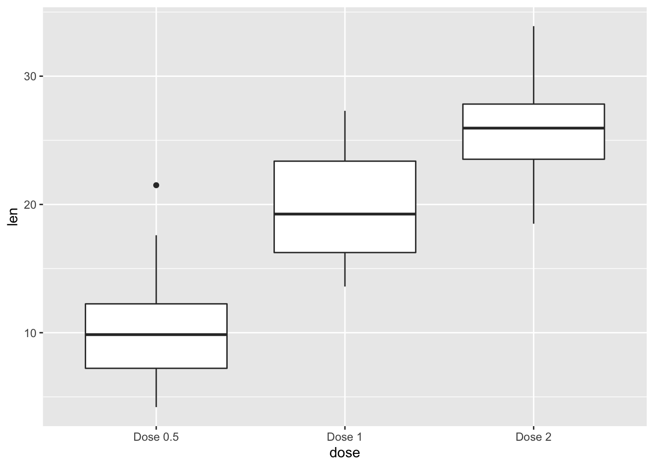
2.21.3 Choose which items to display
p + scale_x_discrete(limits=c("0.5", "2"))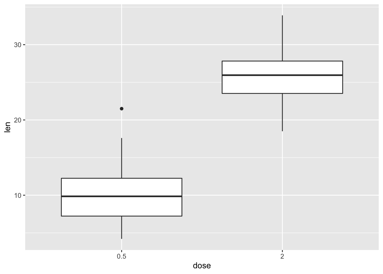
2.21.4 Continuous axes:
2.21.5 Default scatter plot
sp <- ggplot(cars, aes(x = speed, y = dist)) + geom_point()
sp 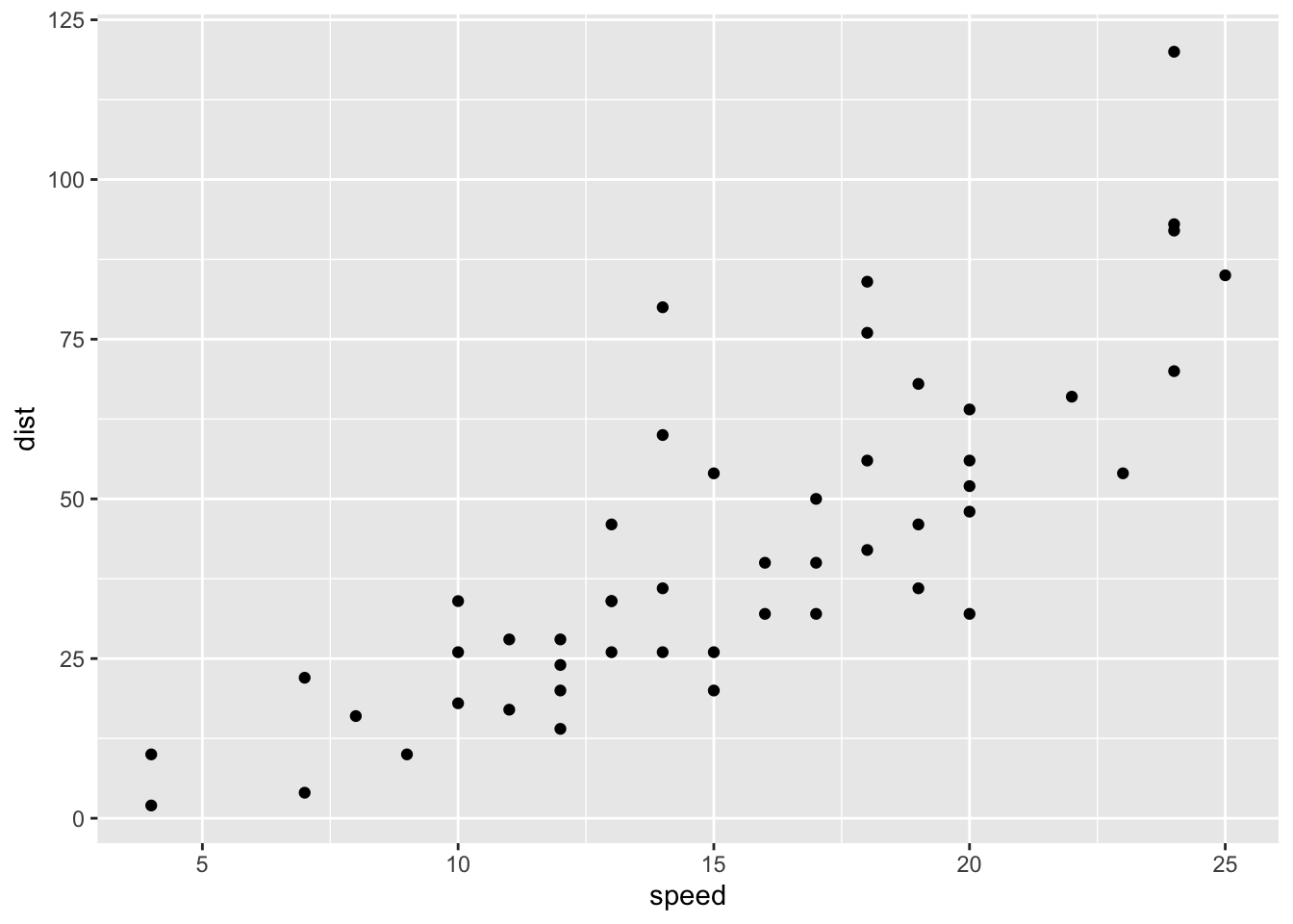
2.22 Customize the plot
2.22.1 1. Change x and y axis labels, and limits
sp <- sp + scale_x_continuous(name="Speed of cars", limits=c(0, 30)) + scale_y_continuous(name="Stopping distance", limits=c(0, 150)) 2.22.2 2. Set tick marks on y axis: a tick mark is shown on every 50
sp + scale_y_continuous(breaks=seq(0, 150, 50)) ## Scale for 'y' is already present. Adding another scale for 'y', which
## will replace the existing scale.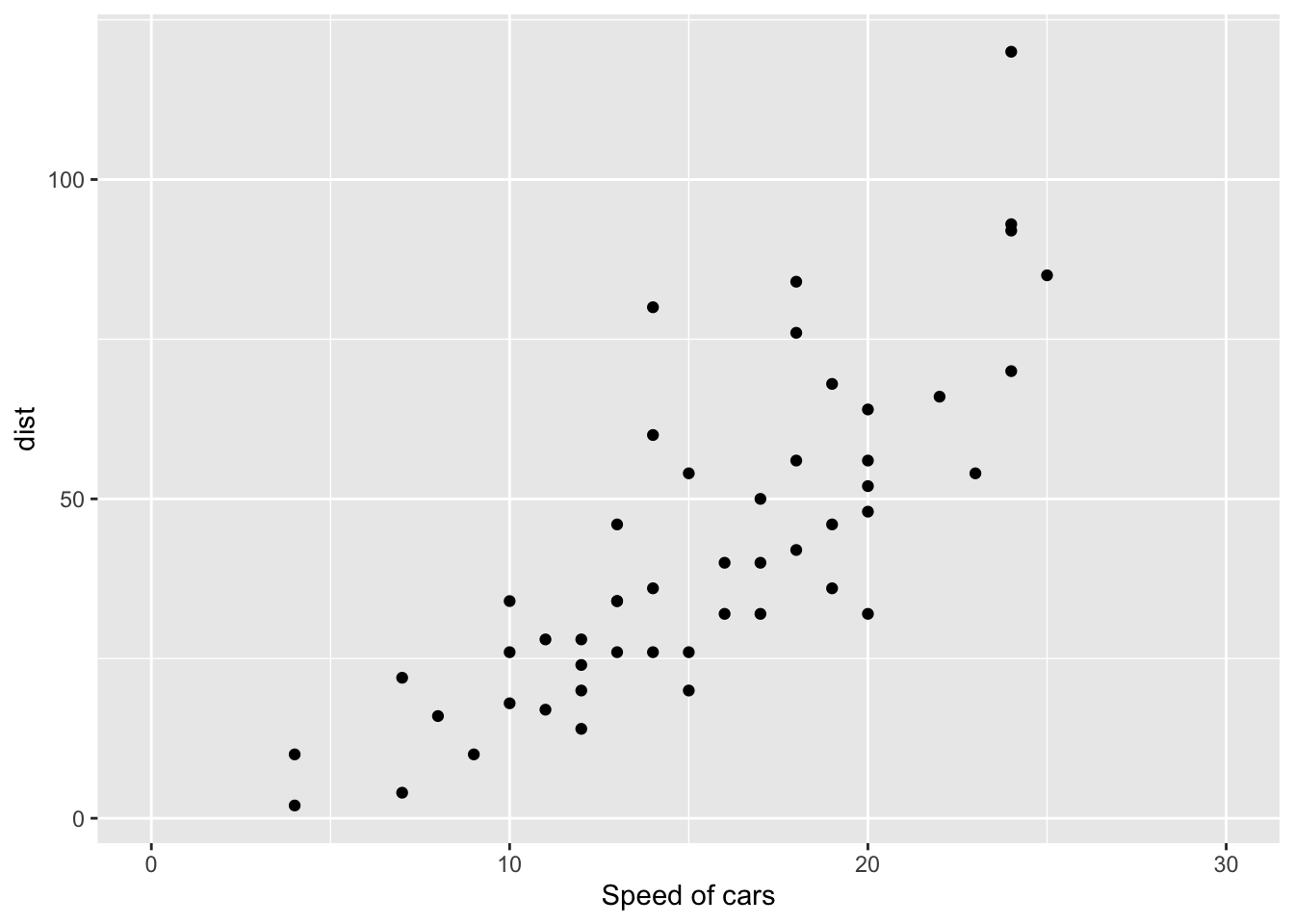
2.22.3 Format the labels
require(scales)
sp + scale_y_continuous(labels = percent) # labels as percents
## Scale for 'y' is already present. Adding another scale for 'y', which
## will replace the existing scale.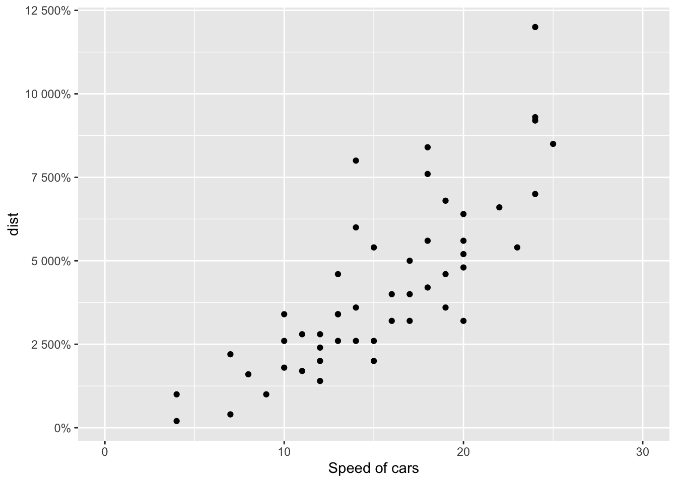
2.23 Add straight lines to a plot: horizontal, vertical and regression lines
2.23.1 Simple scatter plot
sp <- ggplot(data=mtcars, aes(x=wt, y=mpg)) +
      geom_point()
2.23.2 Add straight lines
2.23.3 Add horizontal line at y = 2O; change line type and color
sp + geom_hline(yintercept=20, linetype="dashed", color = "red") 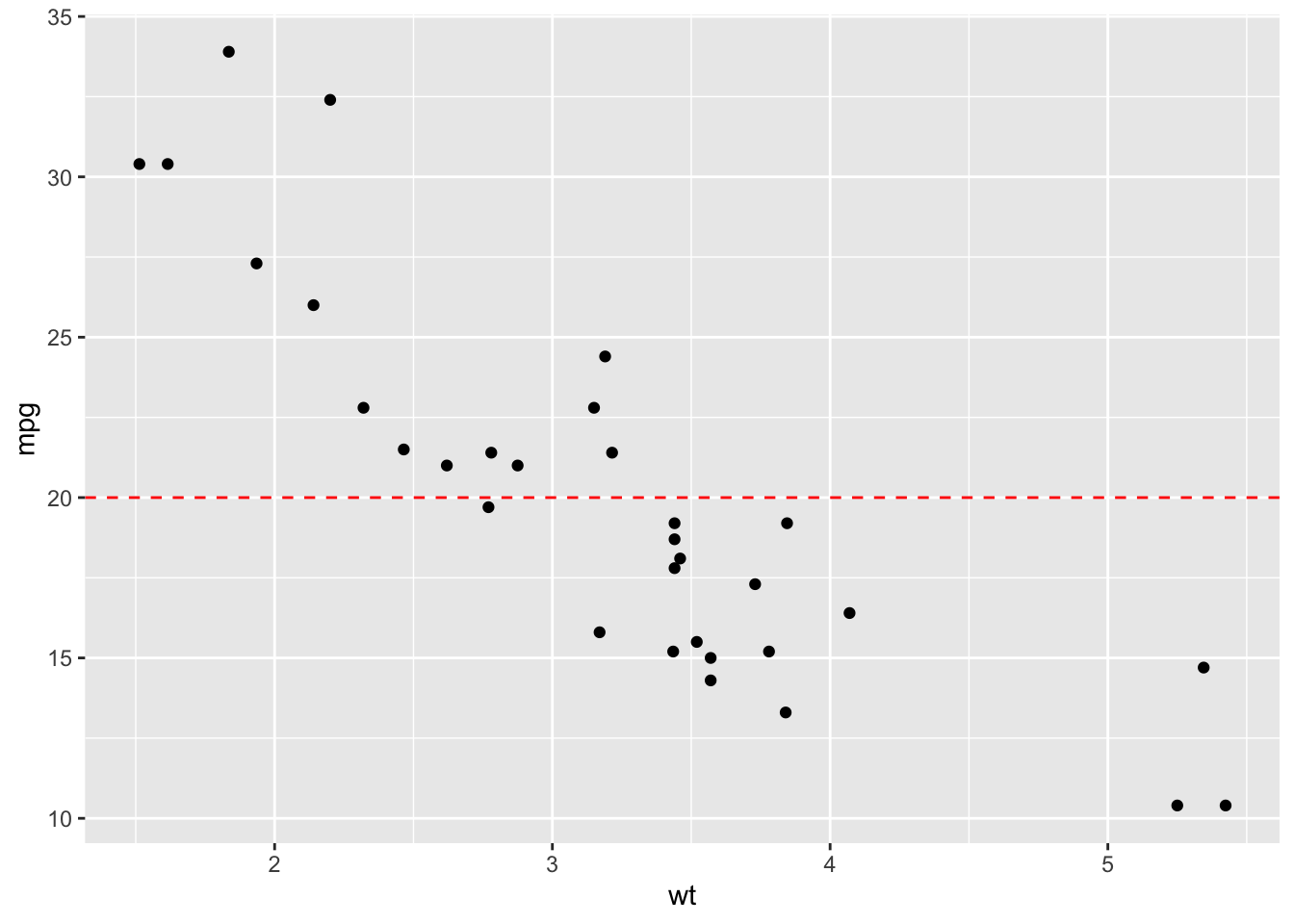
2.24 Add vertical line at x = 3; change line type, color and size
sp + geom_vline(xintercept = 3, color = "blue", size=1.5) 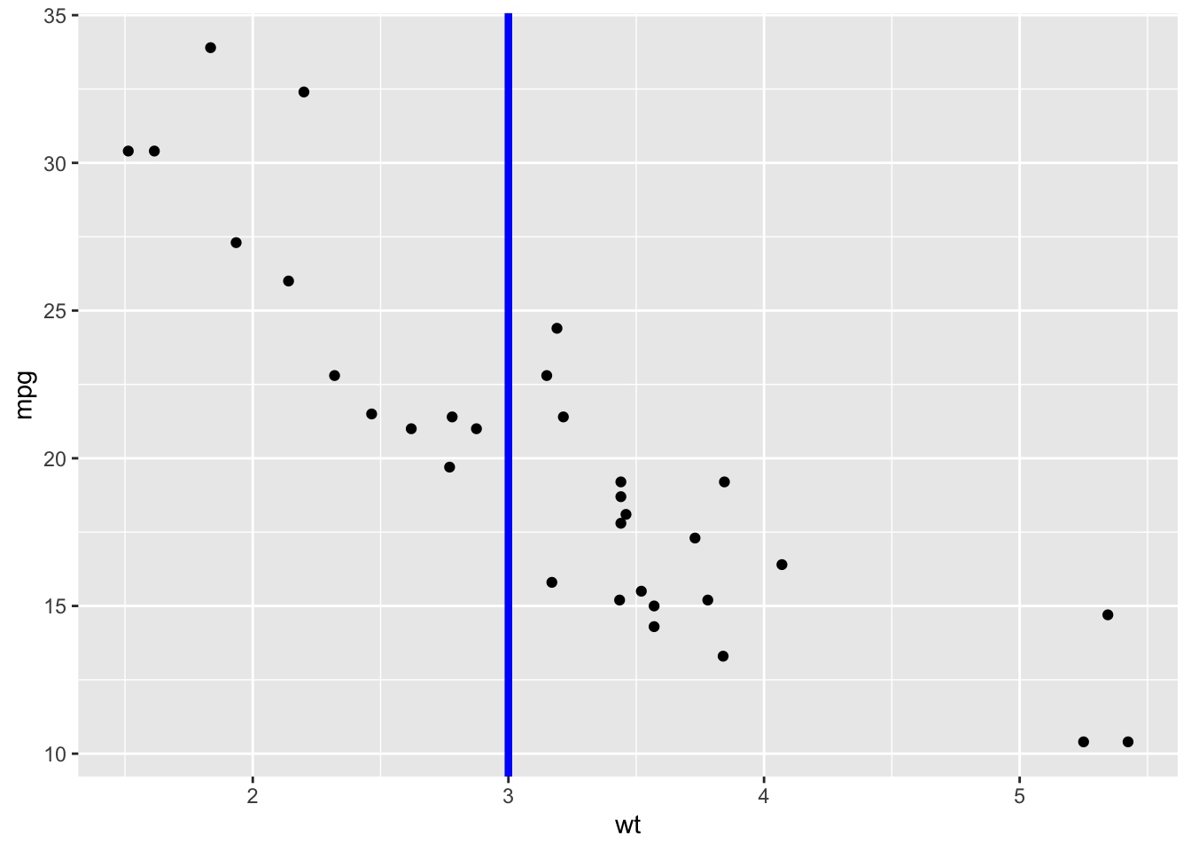
2.25 Add regression line
sp + geom_abline(intercept = 37, slope = -5, color="blue")+ ggtitle("y = -5X + 37") 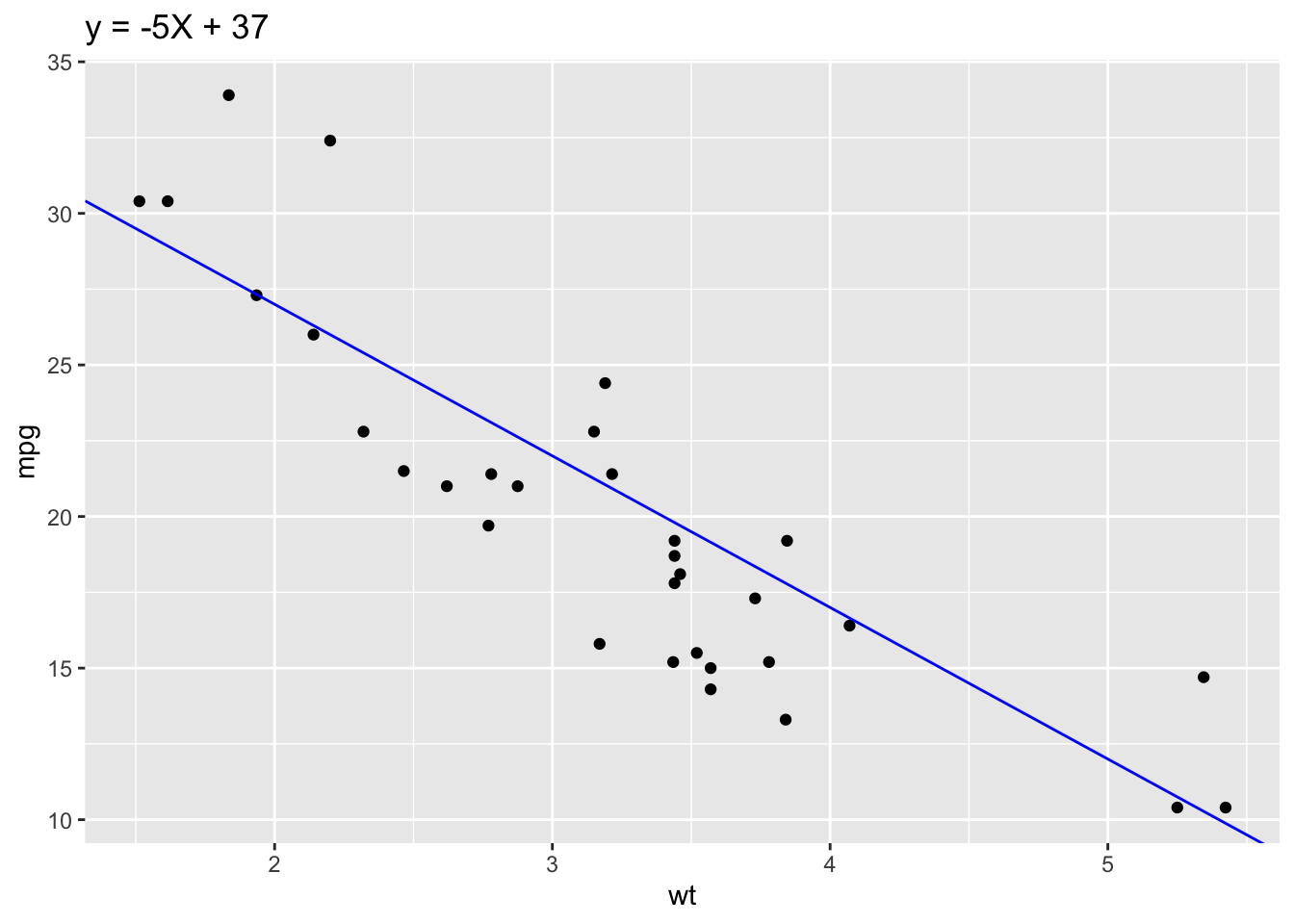
2.26 Add horizontal line segment
sp + geom_segment(aes(x = 2, y = 15, xend = 3, yend = 15))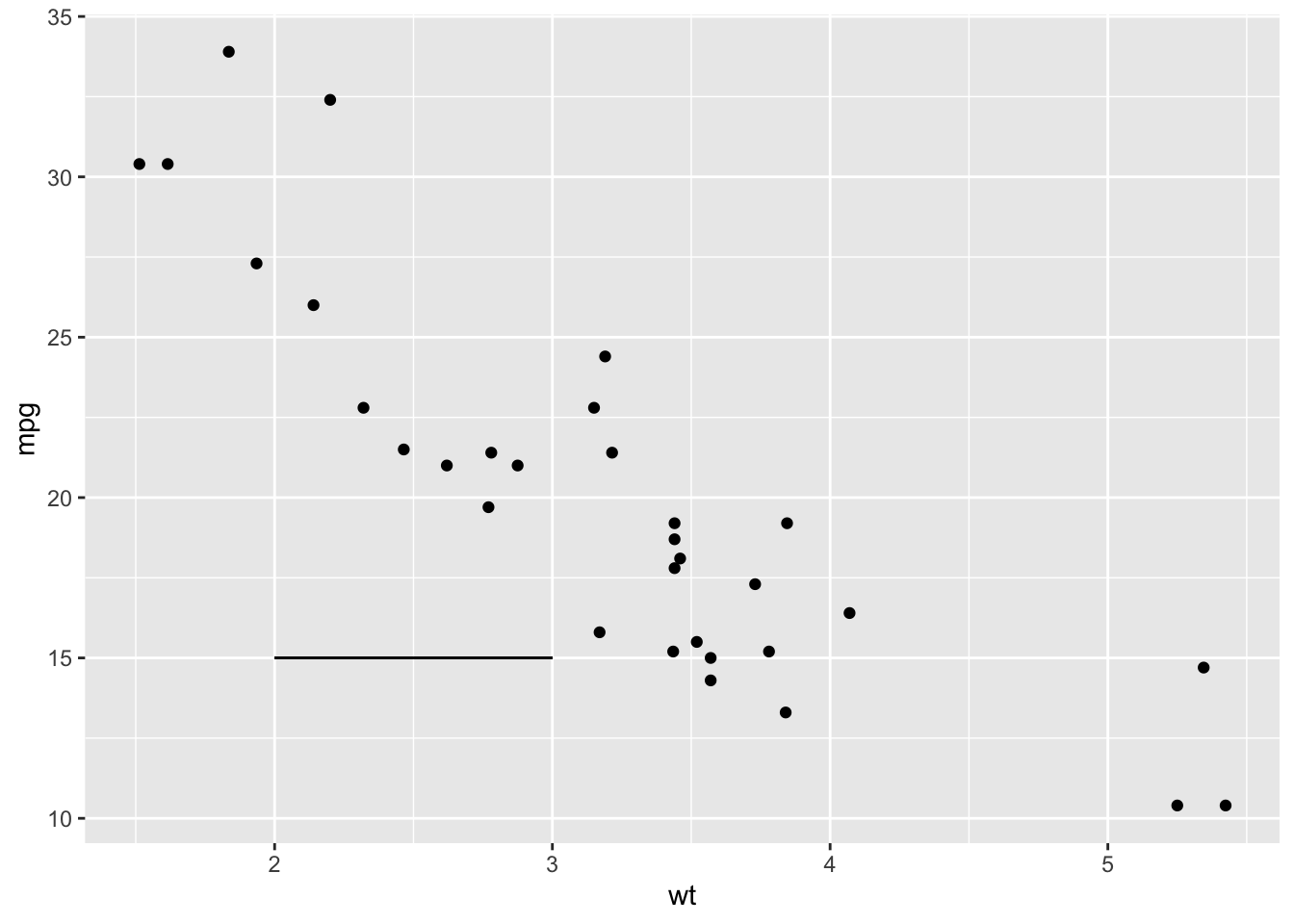
2.27 My Data Example
Water samples were collected on 6/6/18, 9/24/18, 12/17/18, 1/26/19 and ran on an autoanalyzer to determine NO3-N, NH4-N, PO4, and Chl-a concentrations across 8 water tanks identified by treatments (control "A" or nutrient enriched "N"). Moreover this data was used in my master's thesis. Research was conducted at LSU wetland observation greenhouses in Baton Rouge, LA.
2.27.1 Location map
LA_counties <- map_data("county", "louisiana") %>%
  select(lon = long, lat, group, id = subregion)
head(LA_counties, n=3)
## lon lat group id
## 1 -92.61863 30.48136 1 acadia
## 2 -92.48685 30.48709 1 acadia
## 3 -92.48685 30.48709 1 acadiaggplot(LA_counties, aes(lon, lat)) +
geom_point(size = .25, show.legend = FALSE) +
coord_quickmap()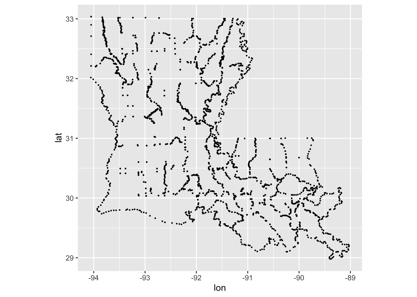
ggplot(LA_counties, aes(lon, lat, group = group )) +
geom_polygon(fill = "white", colour = "grey50") +
geom_point(data = LA_counties, mapping = aes(x = -91.1828669024795, y = 30.4114813833709), colour = "red") +
coord_sf()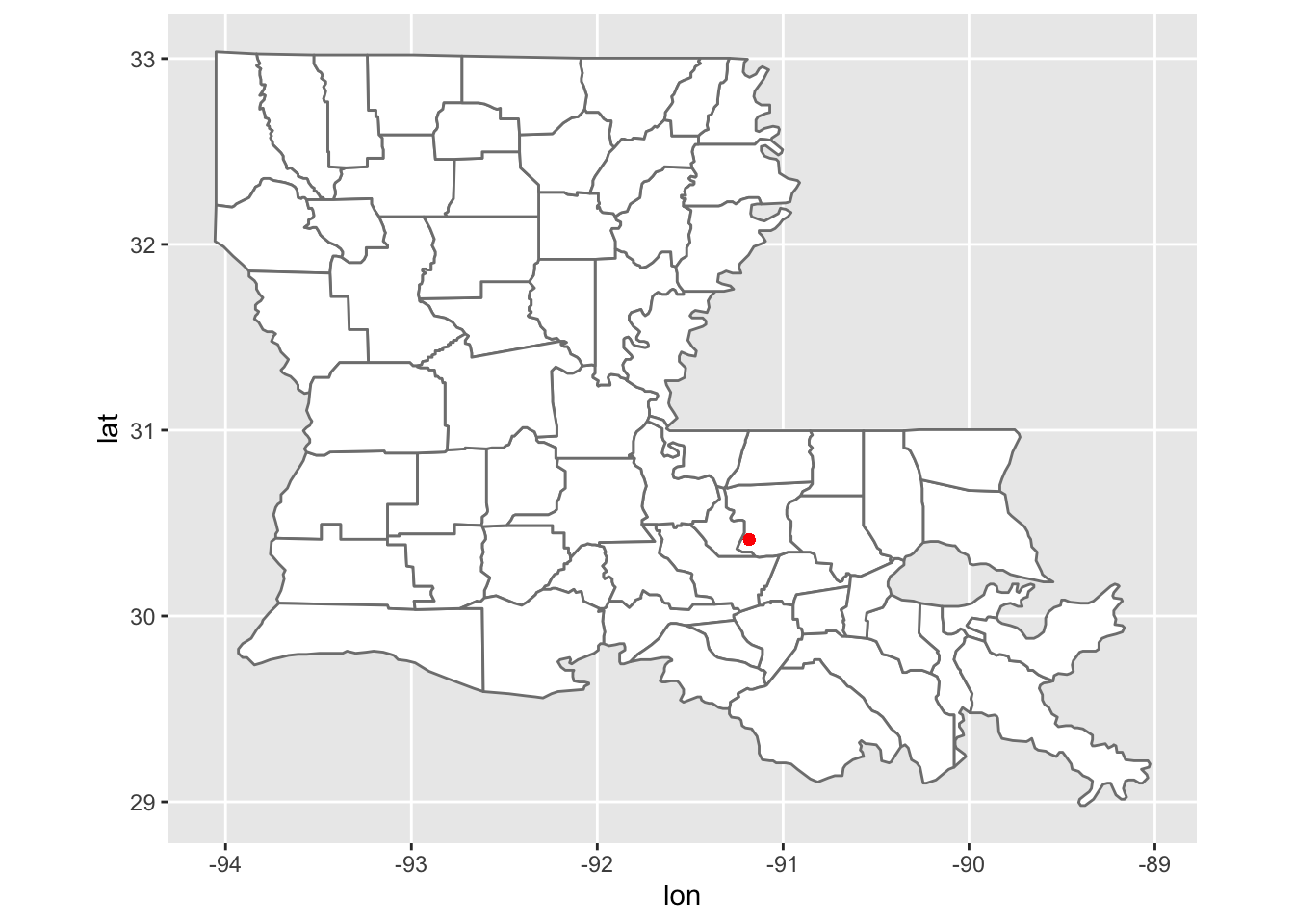 Here I made a map that contains the geolocation of our wetland observation greenhouses using ggplot.
library(readr)
Porewater_data <- read_csv("~/Desktop/R folder/Bookdown/Porewater_data.csv")
head(Porewater_data, n=3)
## # A tibble: 3 x 7
## Tank Date `NO3 (uM)` `NH4 (uM)` `PO4 (uM)` `Conc of chl (ug/… Nutrient
## <dbl> <chr> <dbl> <dbl> <dbl> <dbl> <chr>
## 1 1 6/6/18 2.07 1.35 3.08 2.77 A
## 2 2 6/6/18 4.68 2.48 2.45 5.3 N
## 3 3 6/6/18 3.05 1.77 4.62 2.99 AHere I read the porewater dataset in and headed the first three lines
2.27.2 Scatter plot
ggplot(Porewater_data, aes(x=`Conc of chl (ug/L)`, y=`NH4 (uM)`, group=Nutrient)) + geom_point(aes(shape=Nutrient, color=Nutrient), size=2)+ theme_classic()+ theme(legend.background = element_rect(fill="gray"))+ geom_hline(yintercept=2, linetype="dashed", color = "black")+ geom_abline()+ scale_shape_manual(values=c(3, 16))+ scale_color_manual(values=c('red','blue')) 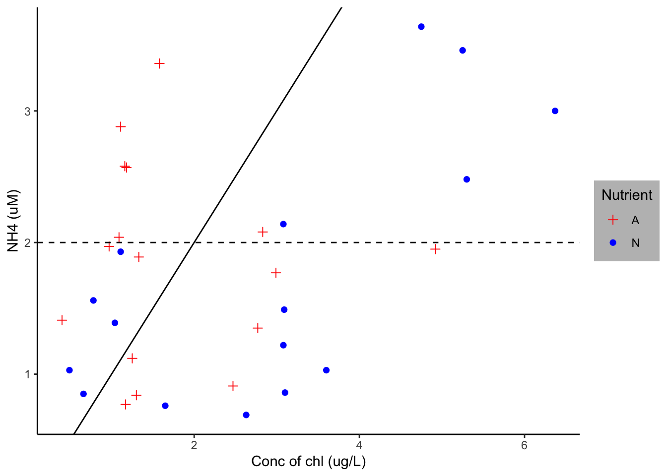
From the porewater dataset, I set x as concentration of chl and y as NH4 and grouped them by nutrients. I then distinguished the nutrient treatments using geom_point, which made them different schapes. I removed the lined background using the theme_classic argument. I added a mid-line and abline using the geom_hline and geom_abline argument respectively. I then manually changed the treatment colors to blue and red.
2.27.3 Scatterplot by date
SamplePoint<-factor(Porewater_data$Date, levels = c("6/6/18", "9/24/18", "12/17/18", "1/26/19"))
ggplot(Porewater_data, aes(x=SamplePoint, y=`NH4 (uM)`, group=Nutrient)) + geom_point(aes(shape=Nutrient, color=Nutrient), size=2)+ scale_shape_manual(values=c(3, 16))+ scale_color_manual(values=c('red','blue'))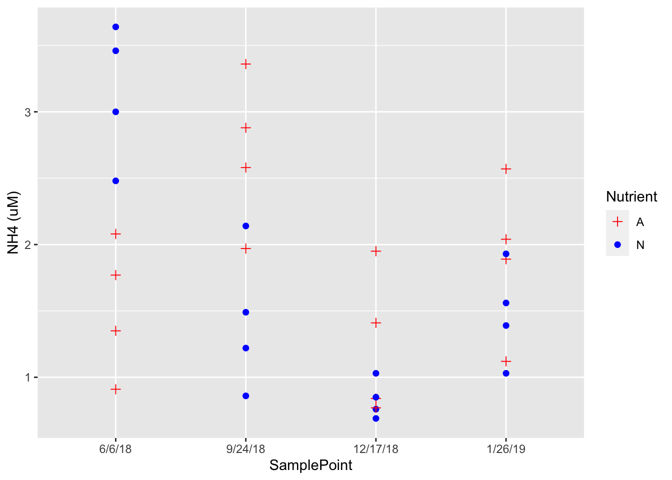
First I made the dates a factor in the porewater dataset in order so they would be distributed simillarly in any future graphs, and named it Sample Point. I replace concentration of chl with Sample point for x, removed the theme, abline and halfline. This data show the scatter distribution of NH4 as it relates to nutrient treatment over 4 time points.
2.27.4 Boxplot
ggplot(Porewater_data, aes(x=SamplePoint, y=`NH4 (uM)`, fill=Nutrient))+ geom_boxplot() + theme_classic()+ labs(fill = "Treatment")+ theme(legend.background = element_rect(fill="gray"))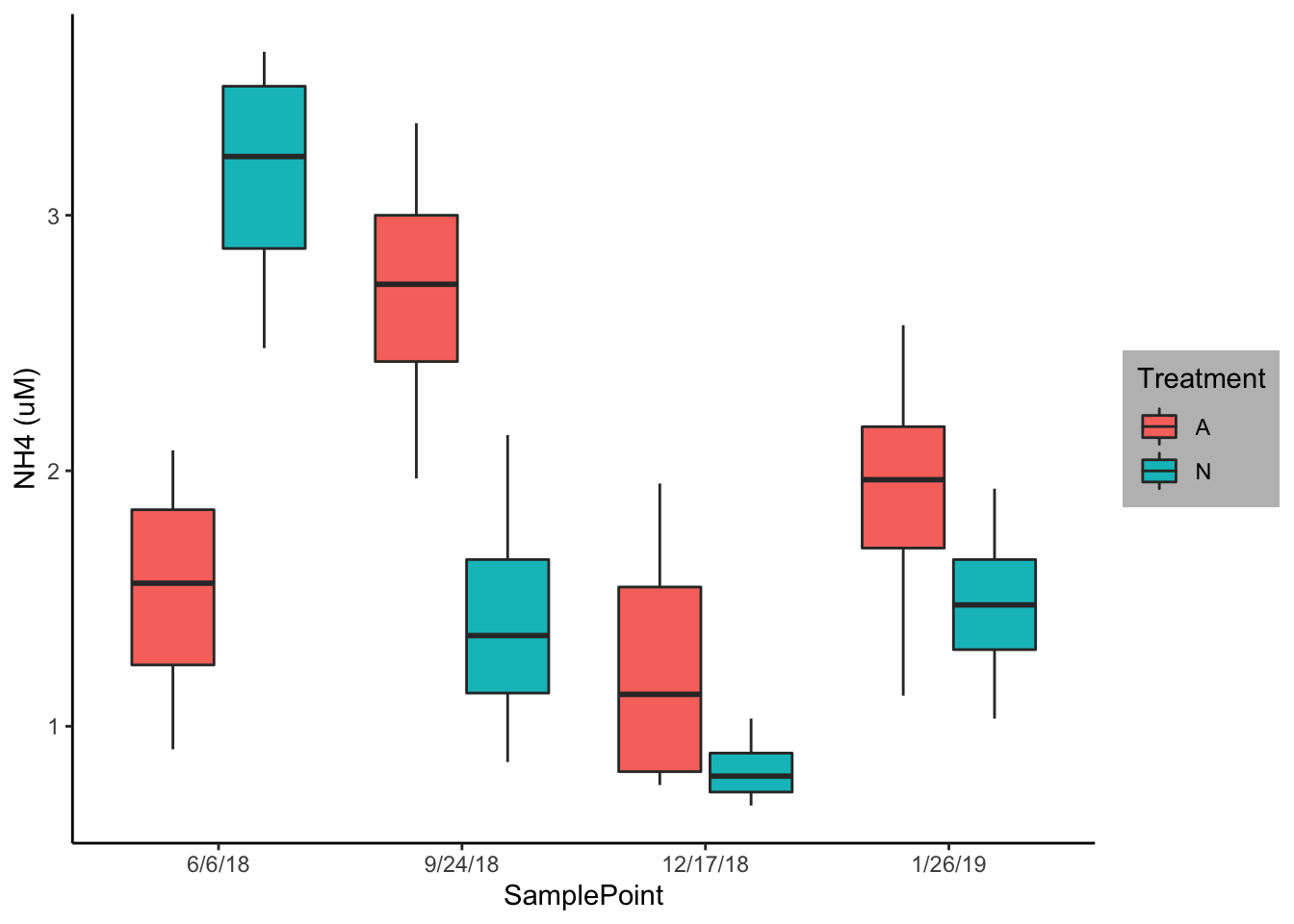
I used the same data construction as above but here I created a boxplot using geom_boxplot. I once again removed the background noise using theme_classic and changed the legend title to treatment. I would most likely use this figure to describe any interaction.