Chapter 8 Nonparametric Functional PCA
In the previous section, we investigated how the assumption that the observed curves of a random function \(X\) live in a finite-dimensional subspace of \(\mathbb{L}^2[0,1]\) simplifies the functional PCA problem. Specifically, by using a known basis \(\Phi\) for this finite-dimensional subspace, we were able to express the process \(X\) as a linear combination of the basis elements, \(X(t) = \Gamma^\mathrm{\scriptscriptstyle T}\Phi(t)\), where now \(\Gamma\) is a random variable in \(\mathbb{R}^b\) which captures all the stochasticity of the process \(X\). In this framwork, the FPCA problem was shown to take the form of a regular multivariate PCA, which facilitated efficient estimation of the eigenfunctions of the covariance operator. We also saw how this exposition lead to intuitive extensions of model-based clustering to the functional data case.
The assumption that all observed paths live in a finite-dimensional subspace spanned by a specific, known basis may not always appropriate, or may be viewed as an overly restrictive inductive bias. For example, one might argue that the assumption of a finite-dimensional path space imposes a limit on the variability and features that the model can represent, and hence biases the model towards solutions in that space. However, without knowing the truth about the generating process, limiting estimated paths to be in a specific space may inadvertantly suppress features that would otherwise be important for downstream tasks. In this chapter we will therefore present an alternative to finite basis expansion, that instead uses kernel smoothing, or local polynomial regression as the backbone for estimating functional principal components.
8.1 Review: Nonparametric Regression
In this section we give a brief overview of kernel smoothing for mean function estimation. Typically, the observed data is assumed to be generated according to, \[\begin{align*} y(t) = f(t) + \epsilon(t), \end{align*}\] where \(y(t)\) is the observed value of the process at time \(t\), \(f(t)\) is the true underlying function which we are interested in estimating, and \(\epsilon(t)\) represents noise, in the sense that it obfuscates the signal \(f(t)\), however it need not be e.g. iid Gaussian at each time point. We will see this later, when we apply this to the specific context of functional data.
Kernel smoothing is a nice approach when one does not want to make strong assumptions about the parametric form of \(f\), instead opting for a “data-driven” estimate of \(f\). In general, a kernel smoother estimates \(f\) at a point \(t\) as a weighted sum of the observed data, \[\begin{equation} \hat{f}(t) = \sum_{i=1}^n w_i(t)y_i, \tag{8.1} \end{equation}\] where the weights \(w_i(t)\) are determined by a so-called kernel, typically denoted by \(\kappa\). If one considers the observed points, \((t_1, \ldots, t_n)\), then the estimate of the function \(f\) at these points is sometimes represented using a smoothing matrix \(S\), \[\begin{equation} \hat{f} = Sy, \tag{8.2} \end{equation}\] where \(\hat{f} = (\hat{f}(t_1), \ldots, \hat{f}(t_n))^\mathrm{\scriptscriptstyle T}\) is the vector of estimated values at the observed time points and \(y = (y_1, \ldots, y_n)^\mathrm{\scriptscriptstyle T}\) is the vector of observed values. In this formulation, each element \(S_{ij}\) of the smoothing matrix therefore represents the weight that the \(j\)th observation contributes to the \(i\)th estimated value \(\hat{f}(t_i)\). The smoothing matrix has many interesting properties and interpretations, which we will look at in more detail when working through some examples later.
A particular kernel smoother is fit by estimating the smoothing matrix \(S\). Generally, a kernel smoother takes the form of a local polynomial regression. That is, we assume that at each point \(t_i\) the true function \(f\) at \(t_i\) is well approximated by a polynomial, \(p_i(t)\). The critical assumption is that the polynomial is different at each point. That is, for a given point \(t_0\) we set, \(\hat{f}(t) = \sum_{j=0}^p \hat{\beta}_j(t-t_0)^j\), where \(\beta = (\beta_0, \ldots, \beta_p)\) is the solution of, \[\begin{equation} \argmin_{\beta} \sum_{i=1}^n \kappa_h(t_0-t_i)\left( y_i - \sum_{j=0}^p\beta_j(t_0-t_i)^j \right)^2. \tag{8.3} \end{equation}\] Here, we have defined \(\kappa_h(u) = \kappa\left(\frac{u}{h}\right)\), where \(\kappa\) is the kernel function and \(h\) is the bandwidth. Notice that the difference \(t_0-t_i\) is passed to the kernel for each difference, so that the weights of the local polynomial regression depend on the proximity of each point \(t_i\) to \(t_0\), rather than the raw value of the points themselves.
In the most general case, the kernel \(\kappa\) can be formed from any function which has finite integral over the reals, \(\int_{\mathbb{R}}\kappa(t)d\mu(t) < \infty\). However, since the kernel determines the weights of a regression, which we want to reflect some sort of locality of the true function at \(t_0\), additional assumptions on the kernel are usually made to facilitate this interpretation. For example, (Hsing and Eubank 2015) suggest the following moment conditions, \[\begin{align*} \int_{\mathbb{R}}t^m\kappa(t)\,d\mu(t) = \begin{cases} 1, & \text{when } m=0, \\ 0, & \text{when } m=1, \\ c \neq 0, & \text{when } m=2, \end{cases} \end{align*}\] which are typically used in practice alongside the assumption of nonnegativity, \(\kappa(t) \geq 0\). It follows that common choices for the kernel \(\kappa\) are symmetric densities with mean \(0\) and finite variance. Some common kernel choices are given below.
- Epanechnikov kernel: \[\begin{align*} \kappa(t) = \begin{cases} \frac{3}{4}(1-t^2), & \text{for } \lvert t \rvert < 1, \\ 0, & \text{otherwise.} \end{cases} \end{align*}\]
- Tukey’s Tricube kernel: \[\begin{align*} \kappa(t) = \begin{cases} (1-\lvert t\rvert ^3)^3, & \text{for } \lvert t \rvert < 1, \\ 0, & \text{otherwise.} \end{cases} \end{align*}\]
- Gaussian kernel: \[\begin{align*} \kappa(t) = \frac{1}{\sqrt{2\pi}}\exp\left( -\frac{t^2}{2}\right). \end{align*}\]
library(ggplot2)

# Kernel functions
epanechnikov = \(t) 0.75*( 1-t^2 )*( abs(t) <= 1 )

tricube = \(t) ( 70/81 )*( (1-abs(t)^3)^3 )*( abs(t) <= 1 )

gauss = \(t) dnorm(t)


# Interval and points for plotting
T = 1e3
t_values = seq( -3, 3, length.out=T )

tibble(
    t = rep( t_values, times=3 ),
    values = c( epanechnikov(t_values), tricube(t_values), gauss(t_values) ),
    Kernel = rep( c("Epanechnikov", "Tricube", "Gaussian"), each=T )
) |>
    ggplot( aes( x=t, y=values, color=Kernel ) ) +
        geom_line( lwd=1.5 ) +
        ggtitle( "Kernel Functions (Scaled to Integrate to 1)" ) +
        xlab("t") + ylab( expression(K(t)) ) +
theme_classic() 
From the plot of the kernels, it is obvious how these define local weighting schemes when considered as a function of the difference \(t_0-t\) for fitting a regression at \(t_0\). As we consider points further away from \(t_0\), the weight of the contribution to the regression gets downweighted, while data points more local to \(t_0\) have more significant weight given to their contribution.
The drop-off of a kernel—the speed with which the weights decrease as we move away form the centre—can additionally be adjusted using the bandwidth, as can be seen by the way the kernel is used for weighting in Equation (8.3). In particular, as \(h\) increases, large deviations are shrunk, and therefore the model gives significant weight to values farther away from \(t_0\), producing a smoother estimate. On the other hand, a smaller value of \(h\) will give significant weight only to those values which are close to \(t_0\), decreasing the overall bias, but since less points are contributing, the variance increases. This is discussed explicitly in Chapter 7 of (Kokoszka and Reimherr 2017).
In practice, one often finds that a local linear model gives good results, and increasing model complexity above that is typically unecessary. We will focus on these in the sequel. It should be noted though that for any choice of polynomial degree, the resulting estimate is given by \(\hat{f}(t_0) = \beta_0\). This can be seen by simply plugging \(t_0\) into the estimated function \(\hat{f}(t) = \sum_{j=0}^p \hat{\beta}_j(t-t_0)^j\). However, (Hsing and Eubank 2015) give an alternative perspective: using the first-order Taylor series expansion we get \(f(t) = f(t_0) + f^\prime(t_0)(t-t_0)\). Matching this with the local linear model shows that \(\beta_0 = f(t_0)\), while \(\beta_1\) gives an estimate of the derivative \(f^\prime(t_0)\). More generally, if one includes a model of higher order, the additional coefficients can be used for derivative estimation (Kokoszka and Reimherr 2017).
As for choosing the bandwidth, this is often done using \(k\)-fold cross-validation. However, this has a tendency to undersmooth the data. As a result, one can use \(k\)-fold cross-validation to find a good value of the bandwidth \(h\) and then adjust it a little bit from there until the estimate is sufficiently smooth to the practioners taste.
# This is a loess example from a previous class
set.seed(12032345)
N <- 300
x <- runif(150, 0,1)
x <- c(x, rnorm(150, 0.5, 0.3))

#
#  A function for the mean of ys
#
mu <- function(x) {
  xrange <- range(x)
  vals <- vector("numeric", length=length(x))
  breaks <- quantile(x, probs=c(1/3,2/3))
  first <- x <= breaks[1]
  second <- (x > breaks[1]) & (x <= breaks[2])
  third  <- x > breaks[2]
  vals[first]  <- -(1 - x[first])^0.5 -0.1
  vals[second] <- sin(x[second] * 4 * pi) + x[second]/10
  vals[third]  <- x[third]^2
  vals
}

y <- mu(x) + rnorm(N, 0, .2)
xrange <- extendrange(x)
yrange <- extendrange(y)
SimulatedData = data.frame(x=x , y=y)

# Using loess function
# uses Tukeys tricube by default

plot(x,y, xlim=xrange,ylim=yrange,
     pch=1, cex=0.7,
     main =  paste0("loess Fit - span=0.75") ,
     cex.axis=1.5 , cex.main=1.5, cex.lab=1.5,
     col=adjustcolor("black" , alpha=0.5)
)
fit <- loess(y~x, data=SimulatedData)

# Get the values predicted by the loess
pred <- predict(fit)
#
# Get the order of the x
Xorder <- order(x)
#
lines(x[Xorder],pred[Xorder], lwd=2, col="steelblue")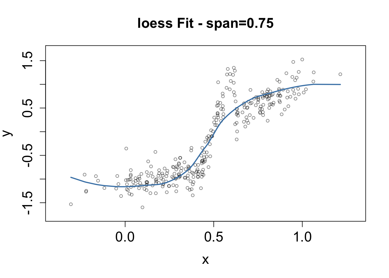
# Now for span=0.15
plot(x,y, xlim=xrange,ylim=yrange,
     pch=1, cex=0.7,
     main =  paste0("loess Fit - span=0.15") ,
     cex.axis=1.5 , cex.main=1.5, cex.lab=1.5,
     col=adjustcolor("black" , alpha=0.5)
)
fit2 <- loess(y~x, span=0.15, data=SimulatedData)
# Get the values predicted by the loess
pred <- predict(fit2)
#
# Get the order of the x
Xorder <- order(x)
#
lines(x[Xorder],pred[Xorder], lwd=2, col="steelblue")
8.2 Sparsely Sampled at Random Time Points
We now want to discuss when kernel smoothing can be used in the context of functional data. We begin with a second-order stochastic process \(X\) that is also a random element of \(\mathbb{L}^2(\mathscr{T})\). We assume that observations of this process take the form, \[\begin{equation} Y_{ij} = X_i(T_{ij}) + \epsilon_{ij}, \quad i \in \mathcal{I} \text{ and } j \in \mathcal{J}_i, \tag{8.4} \end{equation}\] where the \(X_{i}\) are independent replicates of \(X\), and \(T_{ij}\) and \(\epsilon_{ij}\) are iid sampling points and random errors respectively, with \(\mathbb{E}\epsilon_{ij} = 0\) and \(\text{Var}(\epsilon_{ij}) = \sigma^2\). Additionally, it is assumed that the random variables \(\{T_{ij}\}_{i\in \mathcal{I}, j \in \mathcal{J} }\) and \(\{\epsilon_{ij}\}_{i\in \mathcal{I}, j \in \mathcal{J}}\) are independent from one another, and independent of \(X\). Intuitively, this model means that the paths of \(X\) are observed at random and irregular time points, with measurement error. It may sometimes be referred to as a random effects model with a block design. This can be seen by expressing the paths of \(X\) in terms of their eigen expansions so that we have, \[\begin{equation} Y_{ij} = m(T_{ij}) + \sum_{k=1}^\infty Z_{ik}e_k(T_{ij}) + \epsilon_{ij}. \tag{8.5} \end{equation}\]
Under this data model there are two types of designs, which are differentiated by what they assume about the sampling rate of the observed paths. These are dense designs and sparse designs. For dense designs, each path observation is observed at a large number of time points. Hence, although discretely sampled, we still get a rather detailed view of the behaviour of the curve along \(\mathscr{T}\). It follows that for a dense design, the cardnality of \(\mathcal{J}_i\) is large and contains points “densely” spread througout \(\mathscr{T}\). Additionally, for the purpose of asymptotic analysis, it is often assumed that the number of observations per path can increase indefinitely. Then, theoretical results for dense designs are derived under the assumption that observation frequency per path becomes infinitely dense, tending to all of \(\mathscr{T}\).
In contrast to dense designs, sparse designs assume each path is observed at relatively few time points. The points are typically assumed to be irregularly spaced within \(\mathscr{T}\) and different paths are assumed to have observations at different time points. Hence, the cardnality of \(\mathcal{J}_i\) in a sparse design is small for every \(i\) in \(\mathcal{I}\), and it is not required that the points in any \(\mathcal{J}_i\) cover \(\mathscr{T}\). In this case, asymptotic analysis is carried out under the assumption that the cardinality of \(\mathcal{J}_i\) stays bounded by some finite number as the number of sample paths goes to infinity.
8.3 Mean and Covariance Estimation of Functional Data
When we are dealing with data observed according to Equation (8.4) a common approach is to use a kernel smoother to estimate both the mean and covariance function of the data. For the mean estimate we have, \[\begin{equation} (\hat{\beta}_0, \hat{\beta}_1) = \argmin \sum_{i \in \mathcal{I}}\sum_{j \in \mathcal{J}_i} \kappa_h(t_{ij}- t)\left[Y_{ij} - \beta_0 - \beta_1(t_{ij}-t) \right]^2 \tag{8.6} \end{equation}\] from which we get that \(\hat{m}(t) = \hat{\beta_0}(t)\). In (Chen et al. 2017) it is stated that under appropriate regularity conditions, we have \[\begin{align*} \sup_{t \in \mathscr{T}} \lvert m_h(t) - m(t) \rvert = O\left( \left[ \frac{\log n}{n} \right]^{1/2} \right) a.s., \end{align*}\] for dense designs, and \[\begin{align*} \sup_{t \in \mathscr{T}} \lvert m_h(t) - m(t) \rvert = O\left( h^2 + \left[ \frac{\log n}{nh} \right]^{1/2} \right) a.s., \end{align*}\] for sparse designs. These rates are proved in (Hsing and Eubank 2015), in Chapter 8.2. The rate for dense designs is close to the optimal parametric rate, \(O(n^{-1/2})\) as this term grows much faster than \(\log n\). For the sparse rate, we see that the bandwidth now also plays a cruical role along side the sample size. In particular, the term \(h^2\) and \(\frac{\log n}{nh}\) reflect the bias-variance trade off in the sense that, sending \(h\) to zero too quickly will cause the variance of the model to explode (represented by the \(\frac{\log n}{nh}\)) while a conservative choice of \(h\) reflects a stable estimate (i.e. variance disappearing at the parametric rate) that oversmooths as \(n\) increases, failing to capture structural features of the true underlying mean (represented by the \(h^2\) term).
In a similar manner, using the estimate \(\hat{m}_h(t)\) for the mean, we can estimate the covariance function of \(X\), which we denote by \(K(s,t)\). However, some care is needed. First, consider the covariance between two indices of \(Y_{i}\), \[\begin{align*} \text{Cov}(Y_{ij}, Y_{ik} \mid T_{ij},T_{ik}) = \text{Cov}(X_{ij}, X_{ik}) + \sigma^2 \delta_{jk}, \end{align*}\] so that the covariance of \(Y\) is \(K\) plus the additional variance added by the measurement errors. Further, defining the raw covariances as \(k_i(T_{ij}, T_{ik}) = (Y_{ij} - \hat{m}_h(T_{ij}))(Y_{ik} - \hat{m}_h(T_{ik}))\) we have that \(\mathbb{E}\left[ k_i(T_{ij}, T_{ik}) \mid T_{ij}, T_{ik}\right] \approx K(T_{ij}, T_{ik}) + \sigma^2 \delta_{jk}\). It follows that the diagonal term of a smoothed covariance estimate will have a bias. Due to this artifact of measurement error assumption, the diagonal raw covariance terms are typically not considered in estimation of \(K\). That is, we estimate the covariance at position \(\hat{K}(t_1, t_2)\) by solving, \[\begin{align*} (\hat{\alpha}_0&, \hat{\alpha}_1, \hat{\alpha}_2) = \\ &\argmin \sum_{i \in \mathcal{I}}\sum_{j \neq k } \kappa_b(t_{ij}-t_1)\kappa_b(t_{ik}-t_2) \big[ k_i(t_{ij}, t_{ik}) - \alpha_0 - \alpha_1(t_{ij}-t_1) - \alpha_2(t_{ik}-t_2) \big]^2. \end{align*}\]
Then, following (Yao, Müller, and Wang 2005) we estimate the diagonal components by rotating the time domain by 45 degrees. Specifically, we compute the rotated pairwise times, \((T_{ij}^\ast, T_{ik}^\ast)^\mathrm{\scriptscriptstyle T} = R(T_{ij}, T_{ik})^\mathrm{\scriptscriptstyle T}\) where \(R\) is the matrix which rotates \(\mathscr{T}^2\) by 45 degress. Define the estimate of the covariance under this rotated time domain as \(\tilde{K}(s,t)\). Then, since \(K(s,t)\) is a scalar field on \(\mathscr{T}^2\) we have for \(t \in \mathscr{T}^2\), \([RK](t) = K(R^{-1}t)\) and hence, \(\tilde{K}(0, \sqrt{2}t)\) are the estimates for the diagonal terms of the covariance function in the unrotated time domain.
Convergence rates for this estimator are given in (Hsing and Eubank 2015) and (Yao, Müller, and Wang 2005), and one can see that they are very similar to that of the smoothed estimate of the mean.
If one is interested, it is then also possible to estimate the noise variance by first estimating the diagonal terms \(k_i(t_{ij}, t_{ij})\) using a local linear smoother, as with the mean, which we denote by \(\hat{V}(t)\) following (Yao, Müller, and Wang 2005). Then, using the diagonal estimate from the rotated covariance matrix we can estimate \(\sigma^2\) using, \[\begin{align*} \hat{\sigma}^2 = \frac{2}{\lvert \mathscr{T} \rvert} \int \{ \hat{V}(t) - \tilde{K}(t)\} dt. \end{align*}\]
8.4 FPCA and PACE
We can now estimate the eigenpairs of the covariance operator associated with the covariance function of \(X\) in the same way we did in under the finite basis expansion context, by plugging the estimated covariance matrix into the eigenproblem, \[\begin{equation} \int_{\mathscr{T}} \hat{K}(s,t) e_j(t) dt = \lambda_j e_j(s). \tag{8.7} \end{equation}\] However, unlike the finite basis expansion context, we do not get a nice simplification of the problem. Therefore, in practice, this formulation of the eigenproblem is typically solved by discretizing the smoothed covariance, \(\hat{K}(s,t)\). This gives us a matrix representation of the covariance which we can then decompose into eigenpairs using regular PCA. The resulting eigenvectors can then be smoothed to produce eigenfunctions. Let \(\{(\hat{\lambda}_j, \hat{e}_j )\}_{j=1}^b\) be the estimated eigenpairs. Now, our estimation approach guarantees that \(\hat{K}(s,t)\) is symmetric and continuous, but it is not necessarily positive definite. This has the important implication that some of the estimated eigenvalues, \(\hat{\lambda}_j\) may be negative. Hence, it is often advised to take an additional step and project the smoothed covariance matrix onto the space of non-negative definite functions (Chen et al. 2017). This is done by simply dropping the expansion terms associated with negative eigenvalues, i.e. we define a new covariance estimate \[\begin{equation} \tilde{K}(s,t) = \sum_{j \text{ s.t. } \hat{\lambda}_j > 0} \hat{\lambda}_j \hat{e}_j(s)\hat{e}_j(t). \tag{8.8} \end{equation}\] It is shown in (Hall, Müller, and Yao 2008) that under “regularity conditions” \(\tilde{K}(s,t)\) has strictly greater \(\mathbb{L}_2\) accuracy than that of the original estimator \(\hat{K}(s,t)\), i.e., \[\begin{equation} \int_{\mathscr{T}^2} \big\{\tilde{K}(s,t) - K(s,t)\big\}^2 \, d\mu(s)d\mu(t) \leq \int_{\mathscr{T}^2} \big\{\hat{K}(s,t) - K(s,t)\big\}^2 \, d\mu(s)d\mu(t). \tag{8.9} \end{equation}\]
Finally, it is suggested in (Yao, Müller, and Wang 2005) that the number of eigenfunctions to keep, i.e. the implicit basis dimension \(b\), can be chosen using a variant of leave-one-out cross-validation, which they call leave-one-curve-out cross-validation, originally proposed in (Rice and Silverman 1991). In brief, letting \(\hat{m}^{(-i)}\) and \(\hat{e}^{(-i)}_j\) be the mean and eigenfunction estimates after removing the \(i\)th subject from the data, we choose the value of \(b\) that minimizes \[\begin{align*} \text{CV}(b) = \sum_{\in \mathcal{I}}\sum_{i\in \mathcal{J}_i} \big\{ Y_{ij} - \hat{Y}^{(-i)}_{i}(T_{ij}) \big\}^2, \end{align*}\] where \(\hat{Y}^{(-i)}_{i}(t) = \hat{m}^{(-i)}(t) + \sum_{j=1}^b \hat{z}_{ij}^{(-i)}\hat{e}_j^{(-i)}(t)\), with \(\hat{z}_{ij}^{(-i)}\) the estimated scores, which we discuss in the next section.
It is also mentioned in (Yao, Müller, and Wang 2005) that one may also develop an AIC-type criterion for this purpose. Additionally, one can simply use the scree plot of the eigenvalues and choose a cut off such that the retained basis explains a sufficient portion of the data variation.
Chapter 12 of (Kokoszka and Reimherr 2017) gives a decent discussion of the behaviour of these eigenfunctions asymptotically, as does chapter 9 of (Hsing and Eubank 2015).
8.5 Score estimation
Recall that the scores are found from the equation, \[\begin{align*} z_{ij} = \int_{\mathscr{T}}(X_i(t) - m(t))e_j(t)d\mu(t). \end{align*}\] In most of the references we have discussed so far, when the mean, covariance, and eigenfunctions are estimated using kernel smoothing, the scores are estimated by discretizing this integral, i.e. we choose the estimator, \[\begin{equation} \hat{z}_{ij} = \sum_{j \in \mathcal{J}_i}(Y_{ij} - \hat{m}(T_{ij})) \hat{e}_j(T_{ij})\big(T_{ij} - T_{i(j-1)}\big). \tag{8.10} \end{equation}\] Obviously, the quality of this estimator largely depends on the cardinality of \(\mathcal{J}_i\) being large. For sparse data then, this estimator will not give us a good estimate. This issue is what lead (Yao, Müller, and Wang 2005) to proposed the principal components analysis through conditional expectation (PACE) approach.
Consider the \(i\)th sample path, and suppose the time points at which it is sampled, \(T_i = \big(T_{ij}\big)_{j \in \mathcal{J}_i}\) are known, with \(\lvert \mathcal{J}_i\rvert = J_i\). Then, PACE supposes that the associated scores \(Z_{ij}\) and the measurement errors \(\epsilon_{ij}\) are jointly multivariate Gaussian distributed. E.g., letting \(Y_{i}=(Y_{ij})_{j \in \mathcal{J}_i}\) be the observable path points, and \(Z_{ik}\) the \(k\)th score, we have that \((Z_{ik}, Y_i)\) is jointly Gaussian with mean \((0, m(T_i))\) and covariance, \[\begin{align*} \begin{bmatrix} \lambda_k & \lambda_ke_k(T_{i})^\mathrm{\scriptscriptstyle T} \\ \lambda_ke_k(T_{i}) & \Sigma_{Y_i} \end{bmatrix}, \end{align*}\] where we have defined \(\Sigma_{Y_i} = \text{Cov}(Y_i, Y_i) + \sigma^2 I_{J_i}\) and \(\lambda_k e_k(T_{i})^\mathrm{\scriptscriptstyle T} = \lambda_k\big( e_k(T_{i1}), \ldots, e_k(T_{iJ_i})\big)\), and similarly for \(m(T_i)\). Hence, when \(Y_i\) is observed, the best predictor for the score \(z_{ik}\) is the conditional expectation, \[\begin{align*} \mathbb{E}\big[ z_{ik} \mid Y_i \big] = \lambda_ke_{k}(T_i)^\mathrm{\scriptscriptstyle T}\Sigma_{Y_i}^{-1}(Y_i - m(T_i)), \end{align*}\] whose explicit form we derived using the general form of the conditional expectation of a multivariate Gaussian random variable given knowledge of a subset of its components. Since each piece of this expectation is either known or estimable, we use a plug-in estimator to compute the scores, \[\begin{equation} \hat{z}_{ik} = \hat{\lambda}_k\hat{e}_{k}(T_i)^\mathrm{\scriptscriptstyle T}\hat{\Sigma}_{Y_i}^{-1}\big\{Y_i - \hat{m}(T_i)\big\}. \tag{8.11} \end{equation}\] With the scores estimated, the individual trajectories can be recovered, or estimated, as, \[\begin{align*} \hat{X}_i(t) = \hat{m}(t) + \sum_{j=1}^b \hat{z}_{ij}\hat{e}_j(t). \end{align*}\]
8.7 Exercises
None =]