Chapter 2 Function Space Theory
2.1 Setting
In statistics, we are often interested in using samples from some random variable to make inference about aspects of its underlying distribution. This remains true in the context of functional data analysis, however, we need to extend our usual notion of random variable, because an element of \(\mathbb{R}^p\) does not align with our concept of a functional datum. To make this difference explicit, we will usually refer to random variables that take functional values as function-valued random variables or simply random functions. For the purposes of this course, a function-valued random variable will usually be specified as a special kind of stochastic process, with “functional data” arising as collections of paths generated by this process.
Since we cannot hope to develop a fruitful study of random functions without properly defining them, our first order of business is to make the preceeding definition rigourous. In order to do this correctly, one requires knowledge of a fair amount of material that is not typically covered in statistics education unless one goes looking for it. Specifically, most of the material we require falls into the category of functional analysis or stochastic processes. There is also a bit of measure theory involved. In this course, we decide to cover this material, rather than gloss over it, for a number of reasons. First, if one intends to do research in the field of functional data analysis, knowledge of these concepts will usually be needed. Looking back, this is the material I wish I knew going into my study of functional data. Second, covering the material makes the course fairly self-contained—there will by significantly less “trust me bro” kinds of arguments being made. Third, there does not seem to be very many resources which cover this material in the context of functional data, with the textbook I chose for the course being just about the only one. Finally, Dr. Jiguo Cao of SFU offers an extremely good functional data course which covers a lot of the methodological and implementation aspects of functional data. I think the content of this course complements his rather well.
So, in summary, this course will focus mostly on the theoretical underpinnings used by researchers to justify the functional data methods that they concoct. The course will follow the recommended text, (Hsing and Eubank 2015), rather closely. In the last few weeks we will cover material that is a bit more applied in nature. Without further ado, lets get started!
2.2 Metric spaces
As stated in the introduction, we need to extend the definition of a random variable to that of a random function because the elements of \(\mathbb{R}^p\) do not have properties that align with our concept of functional data. Our first order of business is therefore to develop some spaces with elements which serve as better candidates for the modelling of functions. Of course, it will not only be the elements of the space that are of interest, but also the properties of the space, and how these might contribute to the development of methodology for the study of functional data. We begin our search with metric spaces, which will serve as the fundamental building block off of which we will build our function spaces. A definition follows.
Definition 2.1 (Metric Space) Let \(\mathbb{M}\) be a set and \(d: \mathbb{M} \times \mathbb{M} \rightarrow \mathbb{R}\) be a function, called the metric, that satisfies the following properties for all elements \(u\), \(v\), and \(w\) of \(\mathbb{M}\):
- Non-Negativity: The metric \(d\) is non-negative. Formally, \(d(u,v) \geq 0\).
- Identity of Indiscernibles: The metric is zero exactly when its two arguments are equal. Formally, \(d(u,v)=0\) iff \(u=v\).
- Symmetry: The metric takes the same value on two specific points, regardless of the order in which they are passed. Formally, \(d(u,v) = d(v,u)\).
- Triangle Inequality: The metric between two points is never greater than the sum of the metric evaluated between each of these points and some intermediate point. Formally, \(d(u,w) \leq d(u,v) + d(v,w)\).
The pair \((\mathbb{M}, d)\) is then called a metric space. When the metric is known or irrelevant, we may simply represent the metric space using \(\mathbb{M}\). Intuitvely, metrics generalize our notion of distance, e.g. the non-negativity property generalizes the notion that the distance between any two objects should be greater than zero, and the indentity of indiscernibles generalizes the idea that the distance from an object to itself is zero. We now give a couple of common examples of metric spaces.
Example 2.1 (p-dim Reals as a Metric Space) Let \(\mathbb{R}^p\) be the space of \(p\)-dimensional vectors with real entries. For two vectors \(x_1\), \(x_2\) in \(\mathbb{R}^p\) we may define the following function, \[\begin{align*} d(x_1,x_2) = \left(\sum_{i=1}^p (x_{1i} - x_{2i})^2 \right)^{1/2}. \end{align*}\] The function \(d\) satisfies the conditions of a metric, and hence \((\mathbb{R}^p, d)\) forms a metric space. The metric \(d\) is better known as the Euclidean distance.
Example 2.2 (Continuous Functions on Unit Interval as a Metric Space) Let \(C[0,1]\) denote the set of continuous functions on the unit interval of the real line. The Heine-Cantor theorem** tells us that the elements of \(C[0,1]\) are uniformly continuous since \([0,1]\) is compact. The function \(d\) defined as, \[\begin{align*} d(f,g) = \sup_{t \in [0,1]} \left\{ |f(t) - g(t)|\right\}, \end{align*}\] is therefore well-defined for \(f,g\) in \(C[0,1]\). One can show that this function also satisfies the conditions for a metric and hence \((C[0,1], d)\) forms a metric space.
It is also important to notice that it is possible to define various metrics on the same set, and each metric may induce different behaviours on the space. The easiest example of a set with multiple, well known metrics is again Euclidean space, where we commonly see the Euclidean metric, and also the taxi-cab metric.
2.2.1 Properites of Metric Spaces
Even with a metric as our only tool, we can still develop properties which will be important throughout the entirety of the course. We list and briefly discuss them here. You are very likely to have seen all, or many of these, in a previous real analysis and/or linear algebra course.
Definition 2.2 (Open Set) Let \((\mathbb{M},d)\) be a metric space and \(E \subset \mathbb{M}\). Then \(E\) is said to be open if, for each \(x\) in \(E\) we can associated with it an \(\epsilon >0\) such that the set of all points in \(\mathbb{M}\) less than \(\epsilon\) away from \(x\) are also contained in \(E\). That is, \(\{ y \in \mathbb{M} \mid d(x,y) < \epsilon\}\) is a subset of \(E\) for each \(x\) in \(E\).
Intuitively, every point of an open set is an interior point—all other points in the “immediate vicinity” of the point also belong to the open set, where “immediate vicinity” is defined using the metric and \(\epsilon\). The set \(\{ y \in \mathbb{M} \mid d(x,y) < \epsilon\}\) used in Definition 2.2 is commonly called an open ball centered at \(x\), or an epsilon-neighbourhood of \(x\). It is clear from the definition that all open sets in a metric space can be formed from a union of open balls centered at its points.
Definition 2.3 (Closed Set) We say subset \(E\) of \(\mathbb{M}\) is closed if the set \(\{x \in \mathbb{M}\mid x \not\in E\}\) is open.
We can also define the related concept of closure.
Definition 2.4 (Closure) The closure of a subset \(E\) of a metric space \((\mathbb{M}, d)\), denoted by \(\overline{E}\), is the set \[\begin{align*} \overline{E} = \bigcap \big\{ C \subseteq \mathbb{M} \mid C \text{ is closed and } E \subseteq C \big\}. \end{align*}\]
The closure of a set \(E\) can be understood as the smallest closed set in \(\mathbb{M}\) which contains \(E\). Alternatively, one can think of the closure as \(E\) together with all of the limit points of sequences of elements in \(E\).
Definition 2.5 (Dense) A set \(E\) is dense in \(\mathbb{M}\) if \(\overline{E} = \mathbb{M}\).
Essentially, a set is dense in a metric space if every point in the metric space is either in that set, or is arbitrarily close to an element of that set. Probably the most well known example of a dense set is the rational numbers \(\mathbb{Q}\) in the metric space of real numbers, \((\mathbb{R}, \lvert \cdot \rvert)\).
Definition 2.6 (Separable) A metric space \(\mathbb{M}\) is said to be separable if it has a countable, dense subset.
The property of being separable will play an important role in our discussion of Hilbert spaces, as this property directly relates to the existence of an orthonormal basis.
2.2.2 Functions on Metric Spaces
We will often also be interested in functions which map between metric spaces. Of course, properties of such functions, for example smoothness or differentiability, will have direct consequences on what kinds of result can be derived. For example, with continuity, we get that small changes in the input result in small changes in the output which leads to e.g. stability in predictions from fitted models. Differentiability, on the other hand, provide insights into the rate of change of functions, which becomes important when we need to navigate their landscapes, e.g. in optimization.
Definition 2.7 (Continuity) Let \((\mathbb{M}_1, d_1)\) and \((\mathbb{M}_2, d_2)\) be two metric spaces, and let \(f: \mathbb{M}_1 \rightarrow \mathbb{M}_2\) be a function between them. Then, \(f\) is said to be continuous at \(x \in \mathbb{M}_1\) if for every \(\epsilon >0\) there is a corresponding \(\delta_{x,\epsilon} >0\) such that for all \(y \in \mathbb{M}_1\) within distance \(\delta_{x,\epsilon}\) of \(x\) the corresponding function values are less than distance \(\epsilon\) from each other. Formally, \(\forall \epsilon > 0 \,\, \exists \delta_{x,\epsilon} >0\) s.t. \(\forall y \in \mathbb{M}_1\), \(d_1(x,y) < \delta_{x, \epsilon} \,\, \implies \,\, d_2(f(x), f(y)) < \epsilon\).
Definition 2.8 (Uniformly Continuous) A function \(f\) between two metric spaces \((\mathbb{M}_1, d_1)\) and \((\mathbb{M}_2, d_2)\) is said to be uniformly continuous if, for every \(\epsilon >0\) there exists a \(\delta >0\) such that for all pairs of points \(x,y \in \mathbb{M}_1\) that are closer than \(\delta\) to each other, the corresponding function values are less than distance \(\epsilon\) from each other. Formally, \(\forall \epsilon > 0 \,\, \exists \delta >0\) s.t. \(\forall x, y \in \mathbb{M}_1\), \(d_1(x,y) < \delta \,\, \implies \,\, d_2(f(x), f(y)) < \epsilon\).
You are likely to have seen both of these forms of continuity previously, so hopefully you are familiar with them. However, since they will be fundamental to many of the concepts we develop in this course I will provide a basic example to illustrate how they work, and how these two notions of continuity differ.
Example 2.3 (Continuity versus Uniform Continuity) I’m going to choose the function \(f(x) = x^2\) which maps \(\mathbb{R}\) to \(\mathbb{R}\), but the example works with any function that is continuous on the real line, so choose your favorite. As I’ve stated, \(f\) is continuous on \(\mathbb{R}\), and by the Heine-Cantor theorem, it is uniformly continuous on any compact interval. For the sake of illustration, lets consider the interval \([0,1]\) which is closed and bounded and therefore compact, and choose \(\epsilon = 0.19\). Again, any closed and bounded interval and any positive \(\epsilon\) will work, so feel free to choose your favorite. Fortuitously, the derivative of \(f\) is monotonic increasing on \([0,1]\), so for finding the global \(\delta\) associated with \(\epsilon=0.19\), it suffices to look at the function values at the right boundary. The right boundry value is \(x_r = 1\) and we have \(f(x_r)= f(1) = 1\), and the function value that is \(\epsilon\) away from this is \(1-0.19 = 0.81\). Solving \(x^2 = 0.81\) on \([0,1]\) for \(x\), we find \(x=0.9\). Hence, for any \(x \in (0.9, 1)\), \(|f(x_r) - f(x)| < \epsilon = 0.19\). Hence, if \(x\) is within \(\delta = 1-0.9 =0.1\) of \(x_r\), the distance between the function values \(f(x_r)\) and \(f(x)\) will always be less than \(\epsilon\). By the monotonicity of \(df/dx\), \(0.1\) is the largest distance we can find between two function values evaluated at two points within \(\delta\) of each other. Hence, for \(\epsilon = 0.19\), we find that \(\delta=0.1\) is sufficient for meeting the conditions of uniform continuity.
When we instead consider \(f\) on the unrestricted domain \(\mathbb{R}\), it is still continous, but it fails to be uniformly continous. One way to show this is to consider any arbitrary \(\epsilon >0\) and show that for any chosen \(\delta >0\) we can find two points \(x\) and \(y\) which have a distance of less than \(\delta\) from each other, but for which the distance between their function evaluations exceeds \(\epsilon\). That is \(\lvert x-y \rvert < \delta\) and \(|f(x) - f(y)| > \epsilon\). Alternatively, we can show that function evaluations that have a distance greater than \(\epsilon\) can occur on an arbitrarily small interval. This is the route we choose here.
To that end, consider the arbitrary \(\epsilon\) and let \(f(x) = x^2\) and \(f(y)=x^2 + 2\epsilon\) be two function evaluations which are a distance of \(2\epsilon > \epsilon\) apart. Then, \(d(y,x) = (x^2 + 2\epsilon)^{1/2} - x\) and \(\lim_{x\rightarrow \infty} (x^2 + 2\epsilon)^{1/2} - x = 0\). Hence, for any chosen \(\delta >0\) we can always find two points \(x\) and \(y\) which have a distance less than \(\delta\) but for which the distance between their function evaluations exceeds \(\epsilon\). Therefore, \(f(x) = x^2\) is not uniformly continuous on \(\mathbb{R}\).
2.3 Sequences and Emergent Properties of Convergence
Another concept that will be used in nearly every aspect of the course is convergence of sequences within a space. We now define convergence, and a special kind of convergent sequence.
Definition 2.9 (Convergence) Let \((\mathbb{M}, d)\) be a metric space and \(x_n\) a sequence of points in \(\mathbb{M}\). The sequence is said to converge to a limit point \(x \in \mathbb{M}\), denoted by \(x_n \rightarrow x\) if \(d(x_n, x) \rightarrow 0\) as \(n \rightarrow \infty\).
Definition 2.10 (Cauchy Sequence) Let \((\mathbb{M}, d)\) be a metric space and \(x_n\) a sequence of points in \(\mathbb{M}\). The sequence is said to be a Cauchy sequence if \[\begin{align*} \sup_{n,m \geq N} d(x_m, x_n) \rightarrow 0 \quad \text{as} \quad N\rightarrow \infty. \end{align*}\]
Intuitively, a Cauchy sequence is one where the elements of the sequence become arbitrarily close together as the sequence continues. On page 18 of the text (Hsing and Eubank 2015), it is noted that all convergent sequences are necessarily Cauchy, which we can see using the triangle inequality, \(d(x_n, x_m) \leq d(x_n, x) + d(x_m, x) \rightarrow 0\). It is also noted that the converse is not always true, that is, “not all Cauchy sequences are convergent.” The subtlety is that the notion of convergence is usually conditioned on the space of interest. For example, an arbitrary Cauchy sequence of rational numbers does not necessarily converge as a sequence in the rational numbers, but it does converge when considered as a sequence in \(\mathbb{R}\). Our next definition gives a special name to spaces where Cauchy sequences and convergent sequences are synonymous.
Definition 2.11 (Complete) A metric space \((\mathbb{M}, d)\) is said to be complete if every Cauchy sequence is convergent.
As alluded to in the previous comment, \(\mathbb{R}\) is a complete metric space. In the text (Hsing and Eubank 2015) they also show in Theorem 2.1.14 that the set of continous functions on the interval \([0,1]\) is a complete (and separable) metric space under the sup metric. Another property of metric spaces related to convergence of sequences is compactness, which we introduce next.
Definition 2.12 (Compact) A subset \(E\) of a metric space \(\mathbb{M}\) is compact if every sequence in \(E\) has a subsequence which converges to a point in \(E\).
This is the definition of compactness given in the textbook, but this property is better known by the more specific name sequential compactness. Compactness proper is usually defined in terms of finite subcovers of open covers, and is typically used in Topology (e.g. chapter 2 of (Rudin 1976) ). The Bolzano-Weierstrass theorem** is basically a special case of the fact that Definition 2.12, or sequential compactness, is equivalent to the open cover definition of compactness when one is in the context of a metric space. Since metric spaces are the most general kind of space considered in (Hsing and Eubank 2015), we do not run into any issues.
Definition 2.13 (Relatively Compact) A subset \(E\) of a metric space \(\mathbb{M}\) is relatively compact if \(\overline{E}\) is compact.
One should note that relatively compact and compact are not mutually exclusive, e.g. all compact sets are also relatively compact. Additionally, both can still be applied when \(E=\mathbb{M}\), so that it makes sense to talk about a compact/relatively compact metric space.
In terms of completeness and compactness, it may at first be difficult to parse the difference. We can distinguish completeness as a property concerned only with the convergence of Cauchy sequences, while compactness is a statement about all sequences of elements within the space, not just Cauchy sequences. Compactness is therefore a stronger condition than completeness. The two concepts can be connected through the Heine-Borel theorem, which we will state momentarily. First, we need an additional definition.
Definition 2.14 (Totally Bounded) A metric space \((\mathbb{M}, d)\) is totally bounded if for any \(\epsilon >0\) there exists \(x_1,\ldots, x_n\) in \(\mathbb{M}\) such that \(\mathbb{M} \subset \bigcup_{i=1}^n \big\{ x \in \mathbb{M} \mid d(x, x_i) < \epsilon \big\}\) for some finite, positive integer \(n\).
When considering the topological definition of compactness, one can see shades of it in the definition of total boundedness. Since we did not cover the topological definition of compactness, let’s make the difference a bit more explicit. In a totally bounded space, for every small \(\epsilon\), we can completely cover the space using a finite number of open balls with raidus \(\epsilon\). However, in a compact space, any collection of open sets which covers the space contains a finite subcollection which still covers the space—this includes collections of equal-radius open balls as a specific case. Hence, compactness implies total boundedness, but the converse does not generally hold. The next theorem tells us that completeness of the space is the missing link.
Theorem 2.1 (Heine-Borel Theorem) A metric space \(\mathbb{M}\) is compact if it is complete and totally bounded.
The proof is not given in the text, hence it will not be covered. But for those who are curious and have not seen it before, you can find it in (Rudin 1976) as the proof of Theorem 2.41.
2.4 Vector Spaces
Although we were able to derive many interesting and useful properties with only a metric at our disposal, more properties are needed in order for our study of functional data to be sufficiently rich. For example, a chess board can be considered as a metric space under the actions of any piece, but it does not make sense to e.g. add two squares on the board, or scale them by some value. Hence, we now seek to enrich these spaces with an appropriate algebraic structure—the vector space structure.
Vector spaces should be a familiar concept, as linear algebra is a core tool in practically every aspect of statistics. However, for completeness, the rudiment elements are provided in this section.
Definition 2.15 (Vector Space) A vector space \(\mathbb{V}\) over a field \(\mathbb{F}\), is a set of elements, called vectors, for which two operations are defined:
- Vector addition, which is a binary operator \(+: \mathbb{V} \times \mathbb{V} \rightarrow \mathbb{V}\) which takes two vectors \(v_1\) and \(v_2\) to another vector, which we write as \(v_1 + v_2\) in \(\mathbb{V}\).
- Scalar multiplication, is a binary operator \(\cdot: \mathbb{F} \times \mathbb{V} \rightarrow \mathbb{V}\) which takes an element \(a\) of the field \(\mathbb{F}\), called a scalar, and a vector \(v\) in \(\mathbb{V}\) and returns another vector, which we write as \(a\cdot v\).
For \(a_1, a_2\) in \(\mathbb{F}\) and \(v_1, v_2, v_3\) in \(\mathbb{V}\), the two operations are assumed to satisfy the following axioms:
- Addition in commutative, \(v_1 + v_2 = v_2 + v_1\),
- addition is associative, \(v_1 + (v_2 + v_3) = (v_1 + v_2) + v_3\),
- scalar multiplication is associative, \(a_1(a_2v) = (a_1a_2)v\),
- scalar multiplication is distributive with respect to addition \(a(v_1 + v_2) = av_1 + av_2\),
- and with respect to addition in the field \(\mathbb{F}\), \((a_1 + a_2)v = a_1v + a_2v\), and
- the field has an identity element such that \(1v=v\).
In addition, there is a unique element \(0\) with the property that \(v+0=v\) for every \(v \in \mathbb{V}\), and corresponding to each element \(v\) there is another element \(-v\) such that \(v + (-v) = 0\).
Some subsets of vector spaces inherit the vector space structure. We give these important subspaces a specific name.
Definition 2.16 (Linear Subspace) A subset \(A\) of a vector space \(\mathbb{V}\) is a linear subspace, vector subspace, or simply subspace, if \(U\) itself forms a vector space under the operations of \(\mathbb{V}\).
We will usually just refer to linear subspaces as subspaces. As (Hsing and Eubank 2015) note, even if we have a subset \(A\) of a vector space \(\mathbb{V}\) that is not a subspace, we can generate a subspace from \(A\) by considering all finite-dimensional linear combinations of its elements. Here, finite-dimensional means, finitely many elements in the linear combination. This is known as the span of \(A\), and we now formally define this concept.
Definition 2.17 (Span) Let \(A\) be a subet of a vector space \(\mathbb{V}\). The the span of \(A\) is the set containing all the finite-dimensional linear combinations of elements in \(A\).
There is also an another definition of span, which is sometimes just as useful.
Definition 2.18 (Span (Alternate)) Let \(A\) be a subset of a vector space \(\mathbb{V}\). Then the span of \(A\), denoted by \(\text{span}(A)\), is the set, \[\begin{align*} \text{span}(A) = \bigcap \{ U \subseteq \mathbb{V} \mid U \text{ a subspace and } A \subseteq U \}, \end{align*}\] which is the smallest subspace containing \(A\).
The next two concepts are quite important for our study of function spaces, as the existence of a basis will become a crucial component for constructing arguments later on down the road.
Definition 2.19 (Linearly Independent) Let \(\mathbb{V}\) be a vector space and \(B= \{v_{1},\ldots, v_{n} \} \subset \mathbb{V}\). The collection \(B\) is said to be linearly independent if \(\sum_{i=1}^{n} a_i v_i =0\) implies that \(a_{i}=0\) for all \(i\).
Definition 2.20 (Basis) If \(B=\{v_{1}, \ldots, v_{n}\}\) is a linearly independent subset of the vector space \(\mathbb{V}\) and \(\text{span}(B) = \mathbb{V}\), \(B\) is said to be a basis for \(\mathbb{V}\).
A basis is important because it means we can write any \(v\) in \(\mathbb{V}\) as a linear combination of elements in the basis, i.e. \(v = \sum_{i=1}^n a_i v_i\), with each \(a_i\) in \(\mathbb{R}\) (our assumed field).
Definition 2.21 (Dimension) Let \(\mathbb{V}\) be a vector space and \(B\) a basis for \(\mathbb{V}\) which has cardinality \(p < \infty\). Then \(\mathbb{V}\) is said have dimension \(p\) and we write \(\text{dim}(\mathbb{V})=p\).
As noted in the (Hsing and Eubank 2015), if a vector space does not admit a basis with finite cardinality, then it is said have infinite dimension. Most of the spaces that we consider functions to be living in will be naturally infinite-dimensional. However, we will usually make some assumptions about the structure of the space which makes this property manageable.
2.5 Normed Spaces
We now turn our attention to vector spaces on which an additional, useful function, called a norm, is defined.
Definition 2.22 (Norm) Let \(\mathbb{V}\) be a vector space. A norm on \(\mathbb{V}\) is a function \(\lVert \cdot \rVert: \mathbb{V} \rightarrow \mathbb{R}\) which satisfies,
- Non-Negtativity: The norm of a vector is never negative. Formally, \(\lVert v \rVert \geq 0\).
- Positive-Definiteness: Only the zero vector has norm equal to zero. Formally, \(\lVert v \rVert=0\) iff \(v=0\).
- Absolute Homogeneity: Scalar multiplication changes the norm of a vector proportional to the scalar’s magnitude. Formally, \(\lVert av \rVert = |a|\lVert v \rVert\).
- Triangle Inequality: The norm of a sum of two vectors never exceeds the sum of the individual vector norms. Formally, \(\lVert v_{1} + v_{2} \rVert \leq \lVert v_{1} \rVert + \lVert v_{2} \rVert\).
The next theorem connects our earlier section on metric spaces to the previous section on vector spaces, motivating our study of normed spaces.
Theorem 2.2 (A norm defines a metric) Let \(\mathbb{V}\) be a vector space with norm \(\lVert \cdot \rVert\), then \(d(x,y) := \lVert x-y \rVert\) for \(x,y \in \mathbb{V}\) is a metric.
The proof is omitted from the text, but one can show this quite easily by showing that the conditions of Definition 2.1 are satisfied by the candidate metric proposed in Theorem 2.2. It follows that any normed space can be considered as a metric space using the metric defined by the norm. In fact, more is true.
Theorem 2.3 (Finite-Dimensional Normed Spaces are Complete and Separable Metric Spaces) Let \(\mathbb{V}\) be a finite-dimensional normed vector space. Then, \(\mathbb{V}\) is also a complete and separable metric space under any metric generated by a norm on \(\mathbb{V}\).
This is a nice result, but since we will eventually be interested in infinite-dimensional spaces, it is not all that useful. We have included it, because it will help motivate our discussion in the next section. First, in preparation for moving on to infinite-dimensional spaces, we introduce an important synthesis of the property of closure and the span of a subset in a vector space which will be useful in that context.
Definition 2.23 (Closed Span) Let \(A\) be a subset of a normed vector space. The closed span of \(A\) denoted by \(\overline{\text{span}(A)}\) is the closure of \(\text{span}(A)\) with respect to the metric induced by the norm.
In (Hsing and Eubank 2015), a comment is made that the closed span will be important later on as we explore Hilbert spaces, and infinite-dimensional spaces in general. This is true, but their explanation of how to understand the closed span relies on the “including all limit points” definition of closure, which is not how closure is defined in the text. However, the next theorem addresses this issue by making this relationship explicit.
Theorem 2.4 (Composition of Closed Span) Suppose \(A\) is a subset of a separable, complete normed vector space \(\mathbb{X}\). Then, if \(\{ x_n \}\) is dense in \(A\), \(\overline{\text{span}(A)}\) consists of all finite-dimensional linear combinations of the \(x_n\) and the limits in \(\mathbb{X}\) of Cauchy sequences of such linear combinations.
So what is important about the closed span? It might help to recall why the concept of the regular span is important in the finite-dimensional setting. From Theorem 2.3, any finite-dimensional normed vector space is also a complete and separable metric space under a metric generated by a norm. If we consider any subset of a basis for this space, the span of that subset will also form a finite-dimensional normed vector space which is also complete and separable under the same metric. Hence, the span of any subset of basis elements always gives us another space that is of the same type as the original space. However, when we move our attention to infinite-dimensional normed vector spaces which are both complete and separable, this property no longer holds in the general case. In particular, the span of a basis (this has to, of course, be newly defined in the context of infinite-dimensional spaces, but more on that later) for an infinite-dimensional space may not recover the entire space. This is because some elements may only be expressed as infinite series of basis elements, and are therefore not elements of the span. Hence, the space associated with the span is not complete, and we are unable to recover the same type of space that we started with. We get around this issue by instead considering the closed span, which includes limits of sequences in the span, as Theorem 2.4. In this way we are able to include elements of the space which are expressed as infinite series of basis elements. As a result, we are able to use the closed span to generate a space which preserves all the important properties of the original space.
This theorem is also important because it relates the closed span to any dense subset of \(A\). In particular, it follows from this Theorem 2.4 that the closed span of \(A\) is the closure of the set \(\text{span}(\{x_n\})\), and hence that \(\text{span}(A)\) is dense in \(\overline{\text{span}(A)}\).
2.6 Banach Spaces
Although we know from Theorem 2.3 that all finite-dimensional normed vector spaces are complete, this is not necessarily true in the infinite-dimensional case, as the following examples illustrate.
Example 2.4 (Continuous functions with L2 norm) Consider the space \(C[0,1]\) with the norm defined as, \[\begin{align*} \lVert f \rVert = \left( \int_0^1 f^2(t) dt \right)^{1/2}. \end{align*}\] In this context consider the sequence of functions in \(C[0,1]\) generated according to, \[\begin{align*} f_n(t) = (1 -2n \lvert 0.5-t \rvert) I\{t \in E_n\}, \,\, \text{ with }\,\, E_n = [0.5(1-1/n), 0.5(1+1/n)]. \end{align*}\] Then \(f_n\) coverges in this norm to the function which takes the value \(0\) on the entire unit interval except for at \(t=1/2\), where it takes the value \(1\). Hence the sequence is Cauchy, however the limit function \(f\) does not belong to \(C[0,1]\). Thus, \(C[0,1]\) is not complete under this metric.
# Libraries
library(ggplot2)
library(dplyr)
library(tidyr)
library(purrr)

# Create function that will generate any specified fn function
fn = function( n )
{
  bounds = 0.5 * c( (1 - 1/n), (1 + 1/n) )
  f = function(t) # t == the interval [0,1]
  {
    idx = t >= bounds[1] & t <= bounds[2] #where to define nonzero values
    vals = numeric( length(t) )
    vals[idx] = 1 - 2*n*abs( 0.5 - t[idx] )
    return( vals )
  }
  return( f )
}

#Make sure tvals always includes 0.5, for plotting purposes.
# Plot the functions

# Prelims
fnvals = vector( "list", 0L )
tvals  = c(seq( 0, 1, length.out=1000 ),0.5)
nvals  = c( 1, 2, 10, 100 )

# Calculate the fn values
for ( i in seq_along(nvals) ) {
  fnvals[[ i ]] = fn( nvals[i] ) |> (\(u){ u(tvals) })()
}

# reformat for ggplot
fnvals |>
  unlist() |>
  matrix( ncol=length(nvals) ) |>
  t() |>
  as_tibble() |>
  set_names( tvals ) |>
  mutate( n=nvals |> as.factor() ) |>
  pivot_longer( cols = -n, names_to="t", values_to="value" ) ->
  plotdat


# plot
ggplot(plotdat, aes(x = t, y = value, group = n, color=n )) +
  geom_line() +
  labs(title = "", x = "t", y = expression( f[n](t) )) +
  theme_classic() +
  theme(
    axis.ticks.x = element_blank(),
    axis.text.x = element_blank()
  )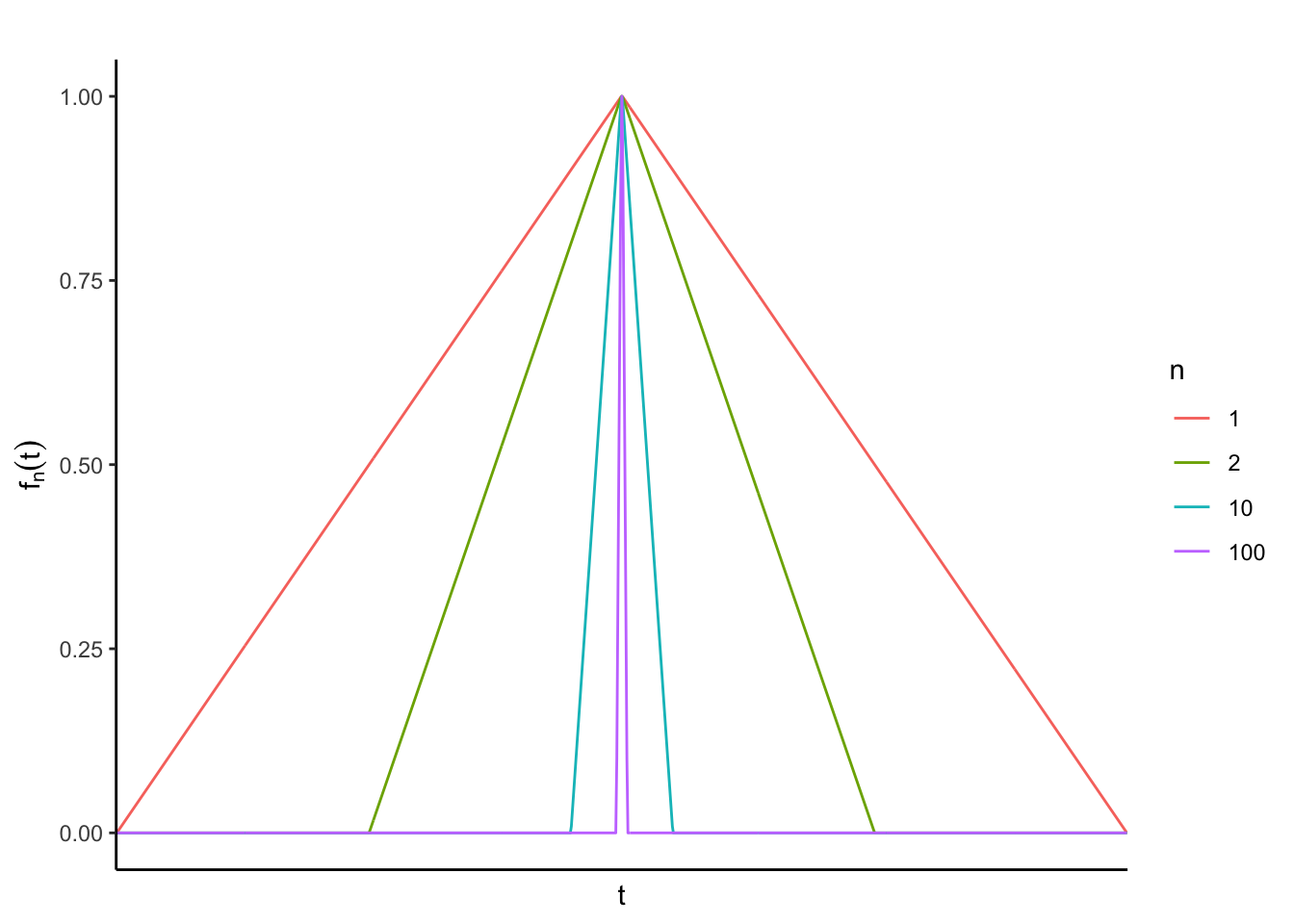
Figure 2.1: A plot showing some of the functions for different values of n.
As we are discovering, completeness is a fairly important concept. As such, we give a special name to normed vector spaces which are also complete metric spaces.
Definition 2.24 (Banach Space) A Banach space is a normed vector space which is complete under the metric associated with the norm.
We’ve already discussed how finite-dimensional normed vector spaces are complete, and hence Banach spaces. Next we give an infinite-dimensional example.
Example 2.5 (C[0,1] with sup norm is complete and separable) In Example 2.4 we saw that \(C[0,1]\) is not a complete space under the norm \(\lVert f \rVert = ( \int_0^1 f^2(t) dt )^{1/2}\). However, when we instead equip this space with the sup norm, \(\lVert f \rVert = \sup_{t \in [0,1]} \lvert f(t) \rvert\) it is complete, as we now show.
Let \(\{f_n\}\) be a Cauchy sequence in \(C[0,1]\) so that, \[\begin{align*} \sup_{m,n \geq N} \lVert f_m - f_n \rVert = \sup_{m,n \geq N} \sup_{t \in [0,1]} \lvert f_m(t) - f_n(t) \rvert \rightarrow 0, \end{align*}\] as \(N \rightarrow \infty\). It follows that for each \(t\) in \([0,1]\) the sequence \(f_n(t)\) is Cauchy in \(\mathbb{R}\), and therefore converges by completeness. Define the pointswise limit \(f(t) = \lim_{n \rightarrow \infty} f_n(t)\). Then, \[\begin{align*} \lvert f_N(t) - f(t) \rvert \leq \sup_{n \geq N} f_n(t) - \inf_{n \geq N} f_n(t) = \sup_{m,n \geq N} \lvert f_m(t) - f_n(t) \rvert, \end{align*}\] which coverges to \(0\) uniformly on \([0,1]\) by assumption. This proves completeness.
By the definition of a dense subset, the definition of separability, and Theorem 2.4, to show separability of \(C[0,1]\) we need to find a countable dense subset \(A\) of \(C[0,1]\) such that for any \(f\) in \(C[0,1]\) there exists a sequence \(f_n\) of elements in \(A\) such that \(\lim_{n \rightarrow \infty} \lVert f_n - f \rVert=0\).
Motivated by the Stone-Weierstrass Theorem** we choose the so-called Bernstein polynomials which, for a specified function \(f\) in \(C[0,1]\) are defined as, \[\begin{align*} f_n(t) = \sum_{i=0}^n \binom{n}{i} t^i (1-t)^{n-i} f(i/n), \end{align*}\] for \(n\in \mathbb{N}\), which is also the degree of the polynomial. Now, fix an arbitrary \(\epsilon >0\). Then by uniform continuity of \(f\) there exists a \(\delta >0\) such that \(\lvert f(x) - f(y) \rvert < \epsilon\) whenever we have \(\lvert x -y \rvert < \delta\). We also define a collection of binomial random variables, \(\{Y_{n,t}\}\) where \(Y_{n,t}\) is distributed according to a binomial distribution with \(n\) trials and probability of success \(t\). We may then write \(f_n(t) =\mathbb{E} f(Y/n)\) and therefore, \[\begin{align*} \lvert f_n(t) - f(t) \rvert &\leq \mathbb{E} \lvert f(Y/n) - f(t) \rvert \\ &= \mathbb{E} \Big[ \lvert f(Y/n) - f(t) \rvert I\big\{ \lvert Y/n - t \rvert \leq \delta \big\} \Big] + \mathbb{E} \Big[ \lvert f(Y/n) - f(t) \rvert I\big\{ \lvert Y/n - t \rvert > \delta \big\} \Big]. \end{align*}\] For the first term, we have \(\mathbb{E} \Big[ \lvert f(Y/n) - f(t) \rvert I\big\{ \lvert Y/n - t \rvert \leq \delta \big\} \Big] \leq \epsilon\) by construction. For the second term, we apply Chebyshev’s inequality to get, \[\begin{align*} \mathbb{E} \Big[ \lvert f(Y/n) - f(t) \rvert I\big\{ \lvert Y/n - t \rvert > \delta \big\} \Big] \leq 2\sup_{y}\lvert f(y) \rvert \frac{\text{Var}(Y)}{n^2\delta^2}, \end{align*}\] where \(\text{Var}(Y) = nt(1-t)\). It follows that \(\mathbb{E} \Big[ \lvert f(Y/n) - f(t) \rvert I\big\{ \lvert Y/n - t \rvert > \delta \big\} \Big] = O(1/n)\) and hence we have, \[\begin{align*} \limsup_{n\rightarrow \infty} \sup_{t \in [0,1]} \lvert f_n(t) - f(t) \rvert \leq \epsilon. \end{align*}\] Since \(\epsilon\) was arbitrary, we are finished.
Of particular interest for us are the collection of Banach spaces known as the \(\mathbb{L}^p\) spaces, which we introduce next. Among these \(L^p\) spaces we will find one in particular which serves as a very popular option for the home of functional data observations.
Definition 2.25 (Lp Space) Let \((E, \mathscr{B}, \mu)\) be a measure space and for \(p\in [1,\infty)\) define the associated \(\mathbb{L}^p\) space, denoted by \(\mathbb{L}^p(E, \mathscr{B}, \mu)\), consists of all measurable functions \(f: E \rightarrow \mathbb{R}\) for which the \(p\)th power of the absolute value is integrable. We define on this space the function \(\lVert \cdot \rVert_p: \mathbb{L}^p(E, \mathscr{B}, \mu) \rightarrow \mathbb{R}\) as \[\begin{align*} \lVert f \rVert_p = \left(\int_E \lvert f \rvert^p d\mu \right)^{1/p}. \end{align*}\] The collection of measurable functions that are finite almost everywhere is denoted by \(\mathbb{L}^\infty(E, \mathscr{B}, \mu)\). On this space we define the function \(\lVert \cdot \rVert_\infty\) as, \[\begin{align*} \lVert f \rVert_\infty &= \text{ess sup}\lvert_{s \in E} f(s) \rvert \\ &= \inf\{ x\in \mathbb{R} \mid \mu(\{ s \mid \lvert f(s)\rvert > x \})\}. \end{align*}\]
The symbols used to define the functions in Definition 2.25 heavily imply that they are norms, but this is not quite true. Specifically, these functions fail positive definiteness because any element \(f\) that takes non-zero values on a set of measure zero will still satisfy \(\lVert f \rVert_\infty =0\). This technically makes them semi-norms rather than norms. In order to make the \(\mathbb{L}^p\) spaces into Banach spaces we consider the quotient space where the equivalence classes are defined to be those functions which differ from each other on a set which has measure \(0\). Specifically, we consider two functions \(f\) and \(g\) to be equivalent and write \(f\sim g\) if the set \(\{x \mid f(x) \neq g(x)\}\) is assigned measure zero by \(\mu\). We then consider the quotient space \(\mathbb{L}^p(E, \mathscr{B}, \mu)/\sim\). Each element of this space is now an equivalance class rather than a single function, and when working with this space we work with class representatives. On this new space, the functions \(\lVert \cdot \rVert_p\) and \(\lVert \cdot \rVert_\infty\) satisfy the conditions to be norms. In the literature, these quotient spaces and their associated norms continue to be denoted by \(\mathbb{L}^p(E, \mathscr{B}, \mu)\), and the norms are referred to as \(\mathbb{L}^p\) norms. We now show that the \(\mathbb{L}^p\) spaces, under this updated definition, are complete, and hence Banach spaces.
Theorem 2.5 (Lp Are Banach) The space \(\mathbb{L}^{p}\) is complete for each \(p \geq 1\).
Proof. We want to show that any Cauchy sequence in \(\mathbb{L}^{p}\) converges to an element of \(\mathbb{L}^p\). The proof in the textbook shows how to do this for \(p \in [1,\infty)\).
Let \(\{f_n\}\) be a Cauchy sequence in \(\mathbb{L}^p\), i.e., \[\begin{equation} \lim_{N \rightarrow \infty} \sup_{m,n \geq N} \lVert f_m - f_n \rVert_p = 0. \tag{2.1} \end{equation}\] It follows that there is an integer subsequence \(n_k\) such that, \[\begin{align*} C := \sum_{k=1}^\infty \lVert f_{n_{k+1}} - f_{n_k} \rVert_p < \infty. \end{align*}\] Through iterative application of Minkowski’s inequality to the function \(\sum_{k=1}^\infty \lvert f_{n_{k+1}} - f_{n_k} \rvert\) we get that, \[\begin{align*} \left\lVert \sum_{k=1}^\infty \lvert f_{n_{k+1}} - f_{n_k} \rvert \right\rVert_p \leq C. \end{align*}\] Finiteness of the norm implies that \(\sum_{k=1}^\infty \lvert f_{n_{k+1}}(s) - f_{n_k}(s) \rvert\) is convergent a.e. \(\mu\). For two indices \(k_1 < k_2\) we can use the triangle inequality to write, \[\begin{equation} \lvert f_{n_{k_2}}(s) - f_{n_{k_1}}(s) \rvert \leq \sum_{j=k_1}^{k_2-1} \lvert f_{n_{k+1}}(s) - f_{n_k}(s) \rvert. \tag{2.2} \end{equation}\] The sum on the right-hand side of this inequality can be made arbitrarily small by making \(k_1\) and \(k_2\) large enough, due to the convergence of the sum in (2.1). In particular, for any \(N\) the partial sum, \(\sum_{k=N}^\infty \lvert f_{n_{k+1}} - f_{n_k} \rvert\) provides an upper bound for all distances of the form \(\lvert f_{n_{k_2}}(s) - f_{n_{k_1}}(s) \rvert\) with \(k_2 > k_1 \geq N\) since the upper bound of this term given in Equation (2.2) is composed of finitely many terms from this sum. Hence, for any \(\epsilon >0\) we can always find an \(N\) such that, \(\sum_{k=N}^\infty \lvert f_{n_{k+1}} - f_{n_k} \rvert < \epsilon\) and therefore \(\lim_{N \rightarrow \infty} \sup_{k_2 > k_1 \geq N} \lvert f_{n_{k_2}}(s) - f_{n_{k_1}}(s) \rvert = 0\) and the sequence \(\{f_{n_k}(s)\}\) is Cauchy and convergent a.e. \(\mu\).
Our candidate limit for the sequence \(f_n\) is then given by, \[\begin{align*} f(s) = \begin{cases} \lim_{k\rightarrow \infty} f_{n_k}(s), & \text{ if the limit exists and is finite,} \\ 0, & \text{otherwise}. \end{cases} \end{align*}\] By the continuity of raising the absolute value to the \(p\)th power, we can write \(\lvert f_n(s) -f(s)\rvert^p = \text{liminf}_{k \rightarrow \infty}\lvert f_n(s) -f{n_k}(s)\rvert^p\), and integrating both sides we get that, \[\begin{align*} \int_E \lvert f_n(s) -f(s)\rvert^p &= \int_E \liminf_{k\rightarrow \infty}\lvert f_n(s) -f_{n_k}(s)\rvert^p \\ &\leq \liminf_{k\rightarrow \infty} \int_E \lvert f_n(s) -f_{n_k}(s)\rvert^p d\mu. \end{align*}\] Setting \(k_1 = n\) and \(k_2 = n_k\) it follows from our previous arguments that for any \(\epsilon >0\) we can choose \(n\) large enough such that \(\liminf_{k\rightarrow \infty} \int_E \lvert f_n(s) -f_{n_k}(s)\rvert^p d\mu < \epsilon\). Hence, \(f\in \mathbb{L}^p\) and \(\lVert f_n - f \rVert_p \rightarrow 0\).
Of particular interest in statistics and measure theory is the case when the underlying measure space is a probability space.
Example 2.6 (Lp Space of Random Variables) Let \((\Omega, \mathscr{F}, \mathbb{P})\) be a probability space. Then \(\mathbb{L}^p(\Omega, \mathscr{F}, \mathbb{P})\) contains random variables defined on \((\Omega, \mathscr{F}, \mathbb{P})\) with \[\begin{align*} \lVert X \rVert_p = \left(\int_\Omega \vert X \rvert^p d\mathbb{P} \right)^{1/p} = (\mathbb{E}\lvert X \rvert^p)^{1/p} <\infty, \end{align*}\] where \(\mathbb{E}\) denotes the expected value.
The following theorem is one of the many reasons that the \(\mathbb{L}^p\) spaces, and one of them in particular, is of interest in the context of functional data analysis.
Theorem 2.6 (Continuous functions dense in Lp) The set of equivalence classes that correspond to functions in \(C[0,1]\) is dense in \(\mathbb{L}^p[0,1]\).
Proof. The proof is given in (Hsing and Eubank 2015) starting at the top of page 30.
2.7 Exercises
2.7.1 Reinforcing Concepts
Exercise 2.1 (d^2 a Metric) The textbook notes that \(d^2\) from Example 2.1 does not satisfy the conditions of being a metric. State the condition it fails and demonstrate its failure.
Exercise 2.2 (Sup Metric) Prove that the sup metric \(d(f,g) = \sup_{t \in [0,1]} \{ |f(t) - g(t)\}\) on the space \(C[0,1]\), as defined in Example 2.2 is indeed a metric.
Exercise 2.3 (Continuity) Show that Definition 2.9 also implies that a function f is continuous at \(x\) if \(f(x_n) \rightarrow f(x)\) whenever \(x_n \rightarrow x\).
2.7.2 Testing Understanding
Exercise 2.4 (Span) Prove that the two definitions of span, Definition 2.17 and Definition 2.18 are equivalent.
Exercise 2.5 (Covergence, Norms, and Completeness) Show that the sequence of functions \(f_n\) in Example 2.4 converges to the specified function \(f(t) = I\{t=1/2\}\) under the \(L^2\) norm. Does \(f_n\) converge to \(f(t) = I\{t=1/2\}\) under the sup norm? If yes, show it. If not, what happens to the sequence under this norm?
2.7.3 Enrichment
Exercise 2.8 (Continuous Convergence and Uniform Convergence) Let \(E\) be a subset of a metric space, and \(f_n\), \(f\) be real-valued functions defined on \(E\). The sequence of functions \(f_n\) are said to converge continuously to \(f\) on \(E\) if, for each \(x\) in \(E\) we have \(f_n(x_n) \rightarrow f(x)\) whenever we have \(x_n \rightarrow x\).
Prove:
- When we have \(f_n\) converging continuously to \(f\), then \(f\) itself is continuous on \(E\).
- If \(f_n\) converges uniformly to \(f\) on \(E\), then we have continuous convergence of this sequence to \(f\), given that \(f\) itself is continuous on \(E\).
- If we further restrict \(E\) to be a compact set, then we have that \(f_n\) converging continuously to \(f\) also implies uniform convergence of \(f_n\) to \(f\).