Chapter 5 Function-Valued Random Variables
In this chapter, we finally characterize function-valued random variables, i.e., random functions. As we have been alluding to in previous chapters, our function space will be a separable Hilbert space \(\mathbb{H}\), almost always taking the form \(\mathbb{L}^2(E, \mathscr{B}, \mu)\), the space of square-integrable functions over a compact metric space \(E\) with respect to measure \(\mu\). A function-valued random variable, denoted in (Hsing and Eubank 2015) by \(\chi\), is a measurable function from some underlying probability space \((\Omega, \mathscr{F}, \mathbb{P})\) to \(\mathbb{H}\). Specifically, \(\chi: \omega \mapsto f\), for \(\omega \in \Omega\) and \(f\in \mathbb{L}^2(E)\). For this function to be measurable, the preimage of each set \(B \in \mathscr{B}\) under \(\chi\) must be in \(\mathscr{F}\). In other words, \(\chi^{-1}(B) := \{\omega \mid \chi(\omega) \in B \}\) is an element of \(\mathscr{F}\). Characterization of this measurability is the subject of our first section.
5.1 Probability Measures on a Hilbert Space
This is concerned with the property of measurability, hence we consider a general separable Hilbert space \(\mathbb{H}\) and let \(\mathscr{B}(\mathbb{H})\) denote the associated Borel \(\sigma\)-algebra. For a particular \(f \in \mathbb{H}\) and \(B \subset \mathbb{R}\) open, let \(M_{f,B}\) be the subset of \(\mathbb{H}\) defined by \(M_{f,B} := \{ g \mid \langle g,f \rangle \in B \}\). Let \(\mathscr{M}\) be the class of all such sets, i.e. \(\mathscr{M} = \{ M_{f, B} \mid f\in \mathbb{H}, B \subset \mathbb{R}, B \text{ open}\}\), and define \(\sigma(\mathscr{M})\) as the smallest \(\sigma\)-algebra containing \(\mathscr{M}\). Our first result is a lemma relating this \(\sigma\)-algebra \(\sigma(\mathscr{M})\) and \(\mathscr{B}(\mathbb{H})\), which we will need for proving our main result of this section.
Lemma 5.1 (Identity of Sigma-Algebras) The \(\sigma\)-algebras \(\sigma(\mathscr{M})\) and \(\mathscr{B}(\mathbb{H})\) are identical.
Proof (sketch). We proceed in the typical fashion of showing \(\sigma(\mathscr{M}) \subset \mathscr{B}(\mathbb{H})\) and \(\sigma(\mathscr{M}) \subset \mathscr{B}(\mathbb{H})\).
Since the inner product is continuous, each set contained in \(\mathscr{M}\) is open (or possibly closed, e.g. when the preimage is all of \(\mathbb{H}\)), hence \(\mathscr{M} \subset \mathscr{B}(\mathbb{H})\).
Since \(\mathscr{B}(\mathbb{H})\) is the smallest \(\sigma\)-algebra containing the open sets, it is sufficient to show that each open set of \(\mathbb{H}\) is contained in \(\sigma(\mathscr{M})\). Do this by constructing an arbitrary open set from a countable union of sets in \(\mathscr{M}\), and the result follows.
Why might we be interested in making a connection between these two \(\sigma\)-algebras? Normally, measurability is defined with respect to the \(\sigma\)-algebra \(\mathscr{B}(\mathbb{H})\), however, due to the previous theorem, we have an equivalence between \(\mathscr{B}(\mathbb{H})\) and \(\sigma(\mathscr{M})\). Hence, every open set generating \(\mathscr{B}(\mathbb{H})\) can be constructed from projections of functions/vectors in \(\mathbb{H}\) onto others. In such a circumstance, we can equivalently characterize measurability in terms of these sets of projections, which turns out to be quite useful, as the next result demonstrates.
Theorem 5.1 (Measurability in a Separable Hilbert Space) Let \(\chi\) be a mapping from some probability space \((\Omega, \mathscr{F}, \mathbb{P})\) to \((\mathbb{H}, \mathscr{B}(\mathbb{H}))\). Then, \(\chi\) is measurable if \(\langle \chi, f \rangle\) is measurable for all \(f \in \mathbb{H}\). Further, if \(\chi\) is measurable, then its distribution is uniquely determined by the (marginal) distributions of \(\langle \chi, f \rangle\) over \(f \in \mathbb{H}\).
There are two typos in the proof of this theorem in (Hsing and Eubank 2015) so we provide the proof here with those typos fixed for the purpose of clarity.
Proof (Part i). (\(\chi\) meas. \(\implies\) \(\langle \chi , f \rangle\) meas.) An immediate consequence of the continuity of \(\langle \cdot,f \rangle\) for each \(f \in \mathbb{H}\).
(\(\langle \chi , f \rangle\) meas. \(\implies\) \(\chi\) meas.) If \(\langle \chi, f\rangle\) is measurable for all \(f\), then for any \(B \subset \mathbb{R}\) open, the set \(\{g \in \mathbb{H} \mid \langle g, f \rangle \in B\} \in \mathscr{M} \subset \mathscr{B}(\mathbb{H})\) satisfies, \[\begin{align*} \chi^{-1}(\{ g \mid \langle g,f \rangle \in B \}) = \{ \omega \in \Omega \mid \langle \chi(\omega),f \rangle \in B\} \in \mathscr{F}, \end{align*}\] where the equality holds by definition, and inclusion in \(\mathscr{F}\) holds by the measurability of \(\langle \chi, f \rangle\) for all \(f \in \mathbb{H}\). This proves the result since the \(\mathscr{M}\) generates \(\mathscr{B}(\mathbb{H})\) by Lemma 5.1.
Proof (part ii, sketch). Define \(\check{\mathscr{M}}\) as the class containing finite intersections of sets in \(\mathscr{M}\) and note that \(\sigma(\check{\mathscr{M}}) = \sigma(\mathscr{M})\). Using the \(\pi-\lambda\) theorem, we can show that this is a determining class, so that if two measures agree on \(\check{\mathscr{M}}\) then they agree on \(\mathscr{B}(\mathbb{H})\).
Let \(M_i\), \(i \in I\) be a finite collection of sets in \(\mathscr{M}\). Then, \(\cap_i M_i \in \check{\mathscr{M}}\) and \(\mathbb{P}\circ\chi^{-1}(\cap_i M_i) = \mathbb{P}(\langle \chi, f_i \rangle \in B_i, i \in I)\), which is a joint probability on the \(\langle \chi,f_i \rangle\). Since \(\check{\mathscr{M}}\) is a determining class, these uniquely define \(\mathbb{P}\circ\chi^{-1}\).
5.2 Mean and Covariance of a Random Element of a Hilbert Space
In this section, we let \(\chi\) be a measurable map from a probability space \((\Omega, \mathscr{F}, \mathbb{P})\) to a separable Hilbert space \(\mathbb{H}\). As such, \(\chi\) is a random function. In this section we will define and discuss the notions of expected value and covariance which generalize the same notions from the multivariate context. Recall that \(\mathbb{E}\lVert \chi \rVert = \int_\Omega \lVert \chi(\omega) \rVert d \mathbb{P}(\omega)\), which is a Lebesgue integral of the random norm over the support of \(\chi\).
Definition 5.1 (Mean of Random Function) If \(\mathbb{E}\lVert \chi \rVert < \infty\), the mean element, or mean, of \(\chi\) is defined as the Bochner integral, \[\begin{align*} m = \mathbb{E}(\chi) := \int_\Omega \chi d \mathbb{P}. \end{align*}\]
Recall from Theorem 3.8 that the condition \(\mathbb{E}\lVert \chi \rVert < \infty\) guarantees Bochner integrability of \(\chi\), and hence the mean element is well-defined. Also notice that by Theorem 4.2 and more explicitly, Example 4.2, we have \[\begin{align*} \mathbb{E}\langle \chi, f \rangle = \langle \mathbb{E}(\chi),f \rangle = \langle m, f \rangle, \end{align*}\] so that \(m\) can also be thought of as the representer of the linear functional \(f \mapsto \mathbb{E}\langle \chi,f \rangle\). Additionally, again using Theorem 4.2 we can show that \(\mathbb{E}\lVert \chi - m \rVert^2 = \mathbb{E}\lVert \chi \rVert^2 - \lVert m \rVert^2\), when \(\mathbb{E}\lVert \chi \rVert^2\) exists and is finite.
In the same way that Definition 5.1 extends the usual understanding of the mean of a random variable to Hilbert space-valued random variables, our definition for the covariance operator seeks to extend the usual notion of covariance for finite-dimensional random variables.
Definition 5.2 (Covariance Operator of a Random Function) Suppose \(\mathbb{E}\lVert \chi \rVert^2 < \infty\). Then the covariance operator for \(\chi\) is the element of \(\mathfrak{B}_{HS}(\mathbb{H})\) given by the Bochner integral, \[\begin{align*} \mathscr{K} = \mathbb{E}\big[(\chi - m) \otimes (\chi - m)\big] := \int_\Omega (\chi - m) \otimes (\chi - m) d \mathbb{P}. \end{align*}\]
Here, the condition \(\mathbb{E}\lVert \chi \rVert^2 < \infty\) and the fact that \(\mathscr{K}\) is an element of \(\mathfrak{B}_{HS}(\mathbb{H})\) also come from an application of Theorem 4.2 and Theorem 3.8, as discussed in Example 4.4. That is, for each \(\omega \in \Omega\) one can define the operator \(T_\omega := (\chi(\omega) -m) \otimes (\chi(\omega) -m)\) and show that the norm of this operator can be specified as \(\lVert T_\omega \rVert_{HS} = \lVert \chi(\omega) - m \rVert^2\). We know this norm is finite whenever \(\lVert \chi(\omega) \rVert^2\) is finite. Hence, if we have \(\mathbb{E}\lVert \chi \rVert^2 <\infty\), then \((\chi - m) \otimes (\chi-m)\) is a random element of \(\mathfrak{B}_{HS}(\mathbb{H})\) and it is Bochner integrable because its Hilbert-Schmidt norm is integrable, i.e., \(\mathbb{E}\lVert \chi - m \rVert^2 < \infty\). It is precisely in such a case that \(\mathscr{K}\) is well-defined. Finally, using the properties of \(\otimes\) and another application of Example 4.4 we can see that \(\mathbb{E}[(\chi - m) \otimes (\chi - m)]= \mathbb{E}(\chi \otimes \chi) - m\otimes m\).
We now derive some properties of the covariance operator \(\mathscr{K}\). Details can be found in (Hsing and Eubank 2015). A notable, although minor, difference is that we include the mean element \(m\) in these results, while (Hsing and Eubank 2015) assumes, without loss of generality, that \(m=0\). We choose to include it simply to make its role in these results explicit.
Theorem 5.2 (Properties of the Covariance Operator) Suppose \(\mathbb{E}\lVert \chi \rVert^2 < \infty\). For \(f,g\) in \(\mathbb{H}\),
- \(\langle \mathscr{K}f, g\rangle = \mathbb{E}\big[ \langle \chi - m,f \rangle \langle \chi - m, g \rangle\big]\)
- \(\mathscr{K}\) is a nonnegative-definite, trace-class operator with \(\lVert \mathscr{K} \rVert_{TR} = \mathbb{E}\lVert \chi - m \rVert^2\), and
- \(\mathbb{P}\big( \chi \in \overline{\text{Im}(\mathscr{K})} \big) = 1\).
Since \(\mathscr{K}\) is a compact, self-adjoint operator, it admits an eigen decomposition as specified in Theorem 4.12, \[\begin{equation} \mathscr{K} = \sum_{j=1}^\infty \lambda_j e_j \otimes e_j, \tag{5.1} \end{equation}\] where the eigenfunctions \(e_j\) form a basis for \(\overline{\text{Im}(\mathscr{K})}\), and the eigenvalues are nonnegative since \(\mathscr{K}\) is also a nonnegative operator. Using the fact that \(\mathbb{P}\big( \chi \in \overline{\text{Im}(\mathscr{K})} \big) = 1\) and Corollary 3.1, we also find that the random function \(\chi\) can be written as \[\begin{equation} \chi = m+ \sum_{j=1}^\infty \langle \chi - m, e_j \rangle e_j = \sum_{j=1}^\infty \langle \chi, e_j \rangle e_j, \tag{5.2} \end{equation}\] with probability 1. This also makes it clear that the one-dimensional projections \(\langle \chi, e_j \rangle\) determine the distribution of \(\chi\). Additionally, this expansion is optimal in terms of the mean squared error: for any natural number \(n\), let \(\chi_n = m + \sum_{i=1}^n \langle \chi - m, e_i \rangle e_i\) be the random function defined as the sum of the first \(n\) terms in the expansion of \(\chi\), then, \[\begin{equation} \mathbb{E}\left[ \lVert \chi - \chi_n \rVert^2 \right] \leq \mathbb{E}\left[ \lVert (\chi - m) - \sum_{j=1}^n \langle \chi-m,f_j \rangle f_j \rVert^2 \right] \tag{5.3} \end{equation}\] where the \(f_j\) are any other orthonormal subset in \(\mathbb{H}\).
5.3 Mean-square Continuous Processes and the Karhunen-Loeve Theorem
In the course introduction it was mentioned that we will view observed curve data as having arisen as realized paths of stochastic processes. In this section, the promised stochastic process view point finally makes its appearance. We first describe in relatively general terms how we can view functional data as having arisen from stochastic processes. We then develop the Karhunen-Loeve (KL) expansion, which is analogous to Equation (5.2) in this new context.
As before, we let \((\Omega, \mathscr{F}, \mathbb{P})\) be a probability space and \((E, \mathscr{B}, \mu)\) be a compact metric space with Borel \(\sigma\)-algebra \(\mathscr{B}\) and finite measure \(\mu\).
Definition 5.3 (Stochastic Process) A stochastic process \(X: E \times \Omega \rightarrow \mathbb{R}\) is a collection of random variables, \(X_t\), indexed by a compact metric space \((E, \mathscr{B})\), each defined on a common probability space \((\Omega, \mathscr{F}, \mathbb{P})\). We write \(X = \{X_t(\cdot) \mid t \in E\}\) where, for each fixed \(t \in E\), \(X_t(\cdot)\) is an \(\mathscr{F}\)-measurable random variable, and for each fixed \(\omega\), \(\{X_t(\omega) \mid t\in E\}\) is a path of \(X\).
Its important to remember that we sort of have three spaces floating around here: the probability space \((\Omega, \mathscr{F}, \mathbb{P})\) on which the random variables are defined, the compact metric space \((E, \mathscr{B}, \mu)\) which serves as the index space for the process, and \((\mathbb{R}, \mathscr{B}(\mathbb{R}))\) which serves as the space in which the random variables (and hence, for us, the resulting functions of interest) are taking values. Keeping these spaces and their roles in order is crucial for understanding these processes.
For a given stochastic process \(X\), if we have existence of the expectations \(\mathbb{E}X_t\) and \(\mathbb{E}(X_sX_t)\) for each \(s,t\) in \(\mathbb{E}\), then we can immediately define the mean and covariance functions of \(X\) as \(m(t) = \mathbb{E}(X_t)\) and \(K(s,t) = \text{Cov}(X_s, X_t)\) respectively. When this holds for a particular stochastic process, we say that it is a second-order process. We will be interested in second-order process with the additional property of mean-square continuity, which we now define.
Definition 5.4 (Mean-Square Continuity) A stochastic process \(X\) is said to be mean-square continuous if, for any \(t \in E\) and any sequence \(t_n\) converging to \(t\) we have that \(\lim_{n \rightarrow \infty} \mathbb{E}\left[ (X_{t_n} - X_t)^2 \right] =0\).
The property of mean-square continuity can be understood as a condition on the continuity of the process in the average sense, rather than on the continuity of any particular path. Intuitively, mean-square continuity tells us that any two points of a path \(X(\omega)\) that have index values which are close with respect to the metric on \(E\) will have values that are close with respect to the metric on \(\mathbb{R}\) as well, on average. This enforces smoothness in the sense that we will usually observe paths which do not have extreme oscillatory behaviours over small regions of the index space.
library(mvtnorm)
library(tibble)
library(ggplot2)
library(ggpubr)

# Preliminaries
nsteps = 500
sig = 0.5

t = seq(0, 1, length.out = nsteps)
Kstgp = outer( t,t,  \(s,t){ exp(- (s - t)^2 / (2 * sig^2)) } ) #K(s,t) for Gaussian process
Kstbm = outer( t,t, Vectorize( \(s,t){ min(s,t) } ) ) #K(s,t) for Brownian motion


# Generate sample paths
set.seed( 90053 )
num_samples = 50
samples_gp = rmvnorm( n = num_samples, mean = rep(0, length(t)), sigma = Kstgp) |> t()
samples_bm = rmvnorm( n = num_samples, mean = rep(0, length(t)), sigma = Kstbm) |> t()
samples_wn = rmvnorm( n = num_samples, mean = rep(0, length(t)), sigma = diag(nsteps)) |> t()

#Alternatively, generate the values together, stack them in df, use facet_wrap on wn, bm label
list(
  "time"  = rep(t, times=num_samples),
  "gp_values" = as.numeric(samples_gp),
  "bm_values" = as.numeric( samples_bm ),
  "wn_values" = as.numeric( samples_wn ),
  "group" = rep(1:num_samples, each=length(t)) |> factor()
) |>
  new_tibble() -> pathsdf

list(
  "time" = t,
  "ymingp" = -2 * sqrt( diag(Kstgp) ),
  "ymaxgp" = 2 * sqrt( diag(Kstgp) ),
  "yminbm" = -2 * sqrt( diag(Kstbm) ),
  "ymaxbm" = 2 * sqrt( diag(Kstbm) ),
  "yminwn" = rep(-2, nsteps) ,
  "ymaxwn" = rep(2, nsteps)
) |>
  new_tibble() -> ci_bounds

# Plotting
gpplot = ggplot() +
  geom_ribbon(data=ci_bounds, aes( x=time, ymin=ymingp, ymax=ymaxgp ), fill="#929292", color="#000000", lty=2, alpha=0.2) +
  geom_line(data=pathsdf, aes(x=time, y=gp_values, group=group, color=group), lwd=0.5) +
  geom_hline(yintercept=0, linetype="solid", color="#000000", lwd=1) +
  labs(title = "",
       x="", y="Gaussian Process Path Value") +
  theme_classic() +
  theme(legend.position = "none")

bmplot = ggplot() +
  geom_ribbon(data=ci_bounds, aes(x=time, ymin=yminbm, ymax=ymaxbm), fill="#929292", color="#000000", lty=2, alpha=0.2) +
  geom_line(data=pathsdf, aes(x=time, y=bm_values, group=group, color=group), lwd=0.5) +
  geom_hline(yintercept=0, linetype="solid", color="#000000", lwd=1) +
  labs(title = "",
       x="", y="Brownian Motion Path Value") +
  theme_classic() +
  theme(legend.position = "none")

wnplot = ggplot() +
  geom_ribbon(data=ci_bounds, aes(x=time, ymin=yminwn, ymax=ymaxwn), fill="#929292", color="#000000", lty=2, alpha=0.2) +
  geom_line(data=pathsdf, aes(x=time, y=wn_values, group=group, color=group), lwd=0.5) +
  geom_hline(yintercept=0, linetype="solid", color="#000000", lwd=1) +
  labs(title = "",
       x="", y="White Noise Path Value") +
  theme_classic() +
  theme(legend.position = "none")

#ggsave("msc_plot.png",ggarrange(gpplot, bmplot, wnplot, ncol=3, nrow=1),width=10, height=5)
ggarrange(gpplot, bmplot, wnplot, ncol=3, nrow=1)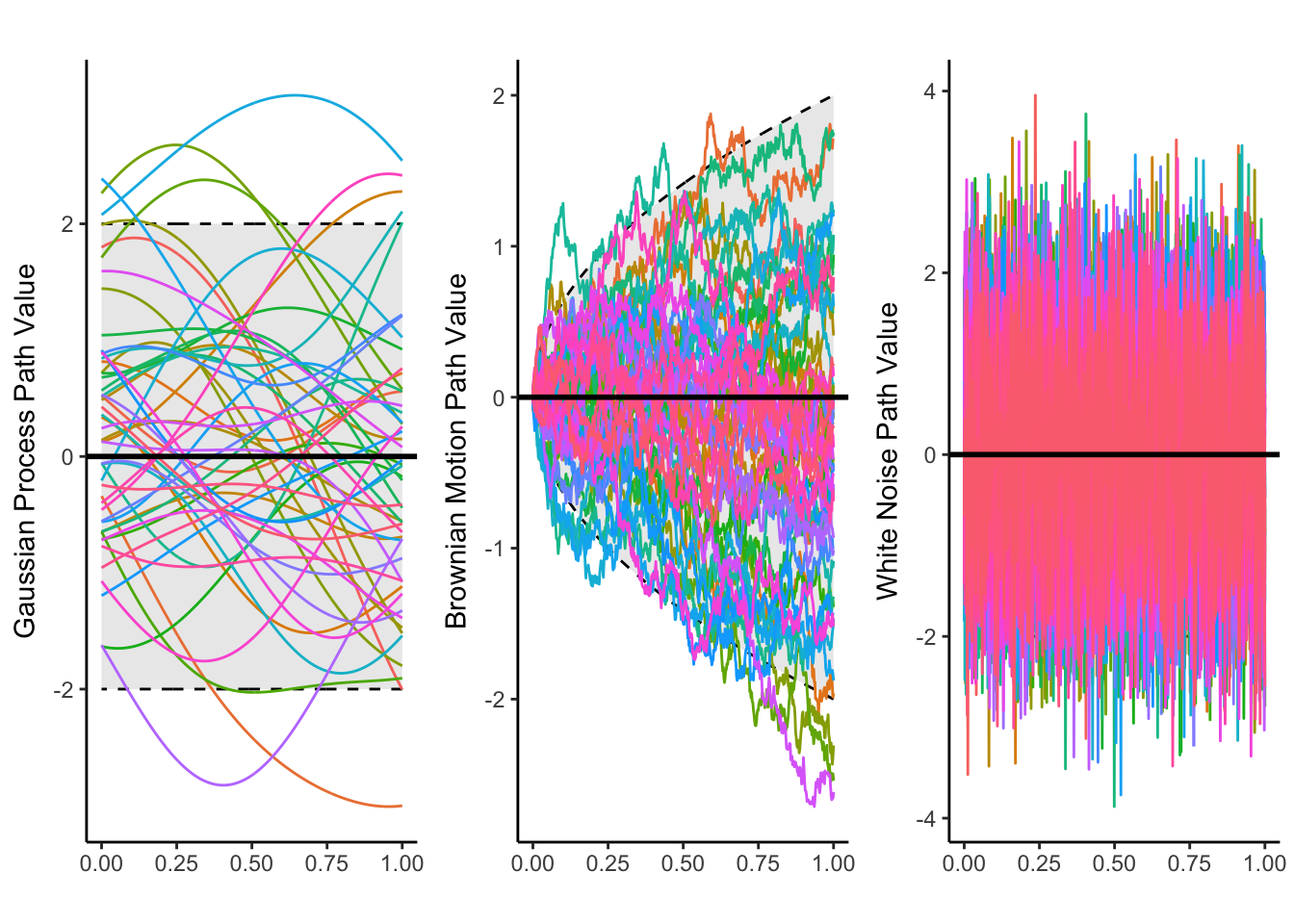
Figure 5.1: A plot showing paths for mean-square continuous processes (left, middle), and a process that is not mean-square continuous (right).
Assuming a process is mean-square continuous is equivalent to assuming its mean function and covariance function are continuous (see theorem 7.3.2 in (Hsing and Eubank 2015)). Despite this, we still cannot guarantee that the resulting paths of a mean-square continuous process \(X\) live in the Hilbert space \(\mathbb{L}^2(E)\), and as a result, we cannot make use of our results from earlier sections without further assumptions or conditions.
In a first step to merging these two view points, we notice that the covariance function \(K\) has all the makings of an integral operator kernel. We have already seen that \(K\) is symmetric and uniformly continuous on \(E\), but we can also show that it is nonnegative in the sense of Definition 4.11. To do this, let \(n\) be any natural number, and \(T_n = \{t_i\}_{i=1}^n\) an arbitrary subset of \(n\) elements in \(E\). We define \(\mathbf{K}\) as the matrix with entries \(\mathbf{K}_{ij} = K(t_i, t_j)\). Then, for any vector \(a\) in \(\mathbb{R}^n\) we have \(\text{Var}(\langle a,X_{T_n} \rangle) = \langle a , \mathbf{K}a \rangle \geq 0\), where with a slight abuse of notation we’ve used \(X_{T_n}\) to denote the vector of random variables \((X_{t_1},\ldots, X_{t_n})\). Then, we know by Mercer’s Theorem that the integral operator on \(\mathbb{L}^2(E)\) defined by \((\mathscr{K}f)(\cdot) = \int_E K(\cdot, s)f(s) d\mu(s)\) has an associated sequence of eigenpairs \((\lambda_j, e_j)_{j \in \mathbb{N}}\) which we can use to write \(K(s,t)=\sum_{j\in \mathbb{N}}\lambda_je_j(s)e_j(t)\), where the sum converges absolutely and uniformly on the support of \(\mu\).
Expansion of the covariance function \(K\) in terms of the eigenpairs of the associated integral operator \(\mathscr{K}\) is the first piece we need for stating and proving the KL expansion. The next, is the notion of an \(\mathbb{L}^2\) stochastic integral of a mean-square continous process, \(X\), which we now define.
First, recall that since \(E\) is a compact metric space, by Theorem 2.1 it is totally bounded. Hence, we can define a function \(D: \mathbb{N} \rightarrow \mathbb{N}\) on the natural numbers \(\mathbb{N}\) such that, for each \(n \in \mathbb{N}\), we can find a partition \(\{E_i\}_{i=1}^{D(n)}\) of \(E\) where each \(E_i\) is in \(\mathscr{B}\) and has diameter less than \(D(n)^{-1}\). Here, the diameter of a set \(E_i\) is 2 times the radius of the smallest open ball, \(\{t \in E \mid d(t,t_i) < r\}\), that contains \(E_i\). In such a case, we can choose an arbitrary element \(t_i\) in each \(E_i\) and define the random function \(G_n(t) = \sum_{i=1}^{D(n)} (X_{t_i}-m_{t_i})I\{t \in E_i\}\), which takes the value \((X_{t_i}-m_{t_i})\) on the partition set \(E_i\) for each \(i\). Then, for any \(f\) in \(\mathbb{L}^2(E)\), we can define the following stochastic integral, \[\begin{align*} \mathscr{I}_X(f; G_n) &= \int_E G_n(s)f(s) d\mu(s) \\ &= \int_E \sum_{i=1}^{D(n)} (X_{t_i}-m_{t_i})I\{s \in E_i\}f(s) d\mu(s) \\ &= \sum_{i=1}^{D(n)} (X_{t_i}-m_{t_i})\int_E I\{s \in E_i\}f(s) d\mu(s) \\ &= \sum_{i=1}^{D(n)} (X_{t_i}-m_{t_i})\int_{E_i}f(s) d\mu(s), \end{align*}\] where we refer to the integral as stochastic due to the randomness of the value \(X_{t_i}\) for each \(t_i\). By this definition, \(\mathscr{I}_X(f;G_n)\) is a random variable, and because \(X\) is a second-order process, \(\mathscr{I}_X(f; G_n)\) is square-integrable and is therefore an element of \(\mathbb{L}^2(\Omega, \mathscr{F}, \mathbb{P})\) for each \(f\) in \(\mathbb{L}^2(E)\) and each choice for the partition/point-representative collection, \(\{(E_i, t_i)\}_{i=1}^{D(n)}\).
Our next goal is to show that the sequence of random variables \(\mathscr{I}_X(f; G_n)\) is Cauchy in \(\mathbb{L}^2(\Omega)\) and hence converges to a particular random variable, which we will denote by \(\mathscr{I}_X(f)\). To do this, we let \(\{E_i\}_{i=1}^n\) and \(\{E_j\}_{j=1}^{n^\prime}\) be two partitions. Then, the sequence is Cauchy if \(\mathbb{E}[\{\mathscr{I}_X(f; G_n) - \mathscr{I}_X(f; G_{n^\prime}) \}^2]\) goes to \(0\) as \(n\), \(n^\prime\) approach \(\infty\). Expanding we get, \[\begin{align*} \mathbb{E}[\{\mathscr{I}_X(f; G_n) &- \mathscr{I}_X(f; G_{n^\prime}) \}^2] =\\ &\begin{aligned} &\sum_{i=1}^{D(n)}\sum_{j=1}^{D(n)} K(t_i,t_j)\mathbb{E}[f; E_i] \mathbb{E}[f;E_j] + \\ &\sum_{i=1}^{D(n^\prime)}\sum_{j=1}^{D(n^\prime)} K(t_i^\prime,t_j^\prime)\mathbb{E}[f; E_i^\prime] \mathbb{E}[f;E_j^\prime] - \\ &2\sum_{i=1}^{D(n)}\sum_{i=1}^{D(n^\prime)} K(t_i,t_j^\prime)\mathbb{E}[f; E_i] \mathbb{E}[f;E_j^\prime], \end{aligned} \end{align*}\] where \(\mathbb{E}[f; E_i] := \int_{E_i} f(s) d\mu(s)\). Each term of this double sum represents the integral of a simple function over the product space \(E \times E\). By increasing \(n\) and/or \(n^\prime\) we see that simple functions, and hence their integrals are becoming closer and closer, so that, each term is approaching the same limit integral, \(\iint_{E\times E} f(s)f(t) d(\mu\times\mu)(s,t)\). For example, considering the first sum, \(\sum_{i=1}^{D(n)}\sum_{j=1}^{D(n)} K(t_i,t_j)\mathbb{E}[f; E_i] \mathbb{E}[f;E_j]\), for any \(\epsilon > 0\), we can choose \(n\) and \(n^\prime\) large enough, i.e. a \(\delta\) small enough, such that \(\lvert K(s, t) - K(t_i, t_j)\rvert < \epsilon\) for all \(s \in E_i\) and \(t \in E_j\). Similar arguments can be made for the other sums. As a result the entire equation tends to \(0\) in the limit.
We now derive some important properties of the limiting random variable \(I_X(f)\).
Theorem 5.3 (Properties of I_x) Let \(X = \{X_t \mid t \in E\}\) be a mean-square continuous stochastic process. The, for any \(f,g\) in \(\mathbb{L}^2(E, \mathscr{B}, \mu)\),
- \(\mathbb{E}[\mathscr{I}_X(f)] = 0\)
- \(\mathbb{E}[\mathscr{I}_X(f)(X_t-m_t)] = \int_E K(s,t) f(s) d\mu(s)\) for any \(t \in E\), and
- \(\mathbb{E}[\mathscr{I}_X(f)\mathscr{I}_X(g)] = \iint_{E \times E} K(s,t)f(s)g(t)d(\mu \times \mu)(s,t)\).
Proof. We prove the first statement. Proofs for the other two are similar.
Since \(E[\mathscr{I}_X(f;G_n)] =0\) for any \(n\), we can write, \[\begin{align*} \lvert E[\mathscr{I}_X(f)] \rvert &= \lvert E[\mathscr{I}_X(f) - \mathscr{I}_X(f;G_n)] \rvert \\ &= \big(\{ E[\mathscr{I}_X(f) - \mathscr{I}_X(f;G_n)] \}^2 \big)^{1/2} \\ &\underset{\text{Jensen's}}{\leq} \big( E\{ [\mathscr{I}_X(f) - \mathscr{I}_X(f;G_n)]^2 \} \big)^{1/2}, \end{align*}\] which goes to \(0\) in the limit, hence we have \(\lvert E[\mathscr{I}_X(f)] \rvert \leq 0\) and the result is proved.
An important corollary of Theorem 5.3, which we will use in the proof of the KL expansion theorem, is that, when \(f=e_i\) and \(g=e_j\) are two eigenvectors of \(\mathscr{K}\), then part 3 of the theorem tells us that \(\mathbb{E}[\mathscr{I}_X(e_i)\mathscr{I}_X(e_j)] = \delta_{ij}\lambda_i\).
Theorem 5.4 (Karhunen-Loeve Expansion) Let \(\{X_t \mid t \in E\}\) be a mean-square continuous stochastic process. Then, \[\begin{align*} \lim_{n\rightarrow \infty} \sup_{t \in E} \mathbb{E}\{ [X_t - X_{n,t}]^2 \} =0, \end{align*}\] where \(X_{n,t} := m_t + \sum_{i=1}^n \mathscr{I}_X(e_j)e_j(t)\).
Proof. \[\begin{align*} \mathbb{E}\{ [X_t - X_{n,t}]^2 \} &= \mathbb{E}[(X_t - m_t)^2] + \mathbb{E}\left[ \left\{\sum_{j=1}^n \mathscr{I}_X(e_j)e_j(t)\right\}^2 \right] - 2 \mathbb{E}\left[\sum_{j=1}^n(X_t -m_t) \mathscr{I}_X(e_j)e_j(t) \right] \\ &= K(t,t) + \sum_{i=1}^n \sum_{j=1}^n \mathbb{E}\left\{\mathscr{I}_X(e_i)\mathscr{I}_X(e_j)\right\}e_i(t)e_j(t) - 2\sum_{j=1}^n \mathbb{E}[(X_t - m_t) \mathscr{I}_X(e_j)]e_j(t) \\ &= \sum_{j=1}^\infty \lambda_j e_j(t)^2 + \sum_{j=1}^n \lambda_j e_j(t)^2 - 2\sum_{j=1}^n \lambda_j e_j(t)^2, \end{align*}\] which tends to zero uniformly on \(E\) by Mercer’s Theorem.
This result has obvious parallels with Equation (5.2), but of course the context is slightly different, which is important. In the next section, we discuss the additional conditions we need to bring these two perspectives together.
5.4 Mean-Square Continuous Process in a Hilbert Space \(\mathbb{L}^2\)
The purpose of this section is to bring together the more abstract random element of a Hilbert space concept, which we built up in the previous chapters and the first section of this chapter, and the stochastic process viewpoint we introduced in the previous section. The idea is to have the stochastic process producing paths which live in a Hilbet space almost surely, and hence allow us to apply our earlier results in this context.
Definition 5.5 (Joint Measurability) A stochastic process \(X\) is said to be jointly measurable if \(X_t(\omega)\) is measurable with respect to the product \(\sigma\)-algebra, \(\mathscr{B} \times \mathscr{F}\). Hence, \(X_{\cdot}(\omega)\) is a \(\mathscr{B}\)-measurable function on \(E\) for all \(\omega\), and \(X_t(\cdot)\) is measurable on \(\Omega\) for each fixed \(t\) in \(E\).
By assuming this additional property, we get the result we are after, as we now show.
Theorem 5.5 (Random Process in L2) Suppose \(X\) is jointly measurable and \(X_{\cdot}(\omega)\) is in \(\mathbb{H}\) for each \(\omega \in \Omega\). then the mapping \(\omega \mapsto X_{\cdot}(\omega)\) is measurable from \(\Omega\) to \(\mathbb{H}\) so that \(X\) is a random element of \(\mathbb{H}\).
Proof (Sketch). Use joint measurability to prove \(\langle X_{\cdot}(\omega), f \rangle\) is a measurable function from \(\Omega\) to \(\mathbb{L}^2(E)\) for each \(f\) in \(\mathbb{L}^2(E)\). This can be done using Fubini’s Theorem. Then appeal to Theorem 5.1.
What is an easily understood condition that implies joint measurability? Consider the next theorem
Theorem 5.6 (Path Continuity Gives Joint Measurability) Assume that for each \(t\), \(X_{t}(\cdot)\) is measurable and that \(X_{\cdot}(\omega)\) is continuous for each \(\omega\) in \(\Omega\). Then, \(X_{t}(\omega)\) is jointly measurable and hence a random element of \(\mathbb{L}^2(E, \mathscr{B}, \mu)\). In this case, the distribution of \(X\) is uniquely determined by the (finite-dimensional) distributions of \(\big(X_{t_1}(\cdot), \ldots, X_{t_n}(\cdot)\big)\) for all \(t_1, \ldots, t_n\) in \(E\), and for all natural numbers \(n\).
(Hsing and Eubank 2015) note that there are many ways to verify sample path continuity, e.g. Kolomogorov’s criterion, which by extension gives us established ways to check for joint measurability. Finally, we give a theorem dedicated to the important properties of a mean-square continuous process which is also a random element of \(\mathbb{L}^2(E, \mathscr{B}, \mu)\).
Theorem 5.7 (Properties of M-S.C. Process in L2) Let \(X = \{ X_t \mid t \in E\}\) be a mean-square continuous process that is jointly measurable. Then,
- the mean function \(m\) of the stochastic process belongs to \(\mathbb{L}^2(E)\) and coincides with the mean element of \(X\) in \(\mathbb{L}^2(E)\) from Definition 5.1,
- the covariance operator \(\mathbb{E}[(X - m)\otimes (X-m)]\) of Definition 5.2 is defined, and coincides with the operator \(\mathscr{K}\) defined as \((\mathscr{K}f)(\cdot) = \int_E K(\cdot, s)f(s) d\mu(s)\) where \(K\) is the covariance function of the process, and,
- for any \(f\) in \(\mathbb{L}^2(E)\), \(\mathscr{I}_X(f) = \int_E X(t)f(t) d\mu(t) = \langle X,f \rangle\).
As a consequence, the scores can be represented as projections onto the basis, as one would typically expect.
5.5 Exercises
5.5.1 Testing Understanding
Exercise 5.1 (Norm of Covariance Component Operator) Verify that the operator \((\chi(\omega) - m) \otimes (\chi(\omega) - m)\) has norm given by \(\lVert \chi(\omega) - m \rVert^2\).
Exercise 5.2 (Mean-Square Continuity) Confirm the claims of the example code, that the Gaussian process with kernel \(\exp\{-1/2(s-t)^2\}\) and Brownian motion are mean-square continuous processes, and show that the white noise process is not mean-square continuous. Do this directly using the definition of mean-square continuity, but also use the equivalent characterization that the mean and covariance functions must be continuous.