4 Basic Syntax (Multi-table Query): JOIN Operations
Now that we have introduced the schematic roles that tables, rows, columns, and keys play in an RDBMS, we can dissect the discuss JOIN operations and their schematic implications for multi-table queries. Afterwards, similar to the approach taken in Basic Syntax (Single-table Query): Clauses and Language Elements, we will step through and analyze an example using the multi-table query from Figure 4.1 with an emphasis on table JOIN operations.
%20with%20clauses%20&%20elements.png)
Figure 4.1: Multi-table Query Example.
Like the previous single-table query example in Basic Syntax (Single-table Query): Clauses and Language Elements the multi-table example in Figure 4.1 contains five clauses (in binding order): i.) FROM, ii.) WHERE, iii.) SELECT, iv.) ORDER BY, and v.) TOP. The most relevant difference with the multi-table query is that it contains the ON/JOIN subclauses; which are subordinated under the FROM clause. Within the ON subclause are the join conditions — most commonly (but not always) an equality between mutual key columns from the source and joined tables — along with the JOIN type. We will elaborate on this simple narrative description in the JOIN Operations subsections below.
4.1 JOIN Operations
There are three different types of JOIN operations in T-SQL: CROSS JOIN, INNER JOIN, and OUTER JOIN. Standard SQL has other join types (e.g., anti-join, natural join) which are not implemented in T-SQL.
While Venn diagrams are a popular means of illustrating JOIN operations, they obscure the row-level logical processing that occurs and only demonstrate the ultimate table product; whereas, viewing input tables and their relationship to the ultimate table product is more informative. To support this approach, discussion about the three types of JOIN operations will refer to the generic data tables in Figure 4.2, in addition to a practical use case for each of the JOIN types.
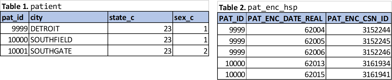
Figure 4.2: Core example tables for discussing JOIN operations.
The first JOIN type to discuss is the CROSS JOIN; not because it is used commonly — in fact, it’s used much less compared with other JOIN types — rather because it’s the simplest syntactically and logically given it does not contain the ON subclause. After, we’ll discuss the JOIN operations that contain the ON subclause (INNER JOIN and OUTER JOIN).
4.2 CROSS JOIN
Takes a source (aka, left) table with n rows and joined (aka, right or destination) table with m rows and produces a table product with n x m rows. CROSS JOIN behaviors create table products that — in relation to the left table — result in the multiplication of rows by a factor of m.
Theoretical Example
As the definition explains, a CROSS JOIN is a combination of all rows from the source and joined tables. Therefore, there are no join conditions and no ON subclause. To help visualize the CROSS JOIN operation, see the example query below, which uses Tables 1 and 2 from Figure 4.2: patient table (master file of all patients in Clarity) and pat_enc_hsp table (master file of all facility patient encounters in Clarity).
SELECT
  pats.pat_id,
  pats.city,
  pats.state_c,
  pats.sex_c,
  encs.pat_id,
  encs.pat_enc_date_real,
  encs.pat_enc_csn_id
FROM patient AS pats
  CROSS JOIN pat_enc_hsp AS encs
The input/output from the above query is shown in Figure 4.3. Table 1 (patient) is the source/left table and Table 2 (pat_enc_hsp) is the joined/right table. The red arrows from patient illustrates the first row’s linkage to all rows in Table 2, an operation that essentially occurs for each row of Table 1, producing the n x m table product (i.e., 3 x 5 = 15). Realistically, this join scenario has little, if any practical value; which is why CROSS JOINS are less common. The most common scenario for CROSS JOIN’s is creating tables of integers for use in more advanced queries, which implicates more complex syntax and so will be deferred to later examples in this manual. A more accessible example (albeit not a pure CROSS JOIN) is discussed in the next section.
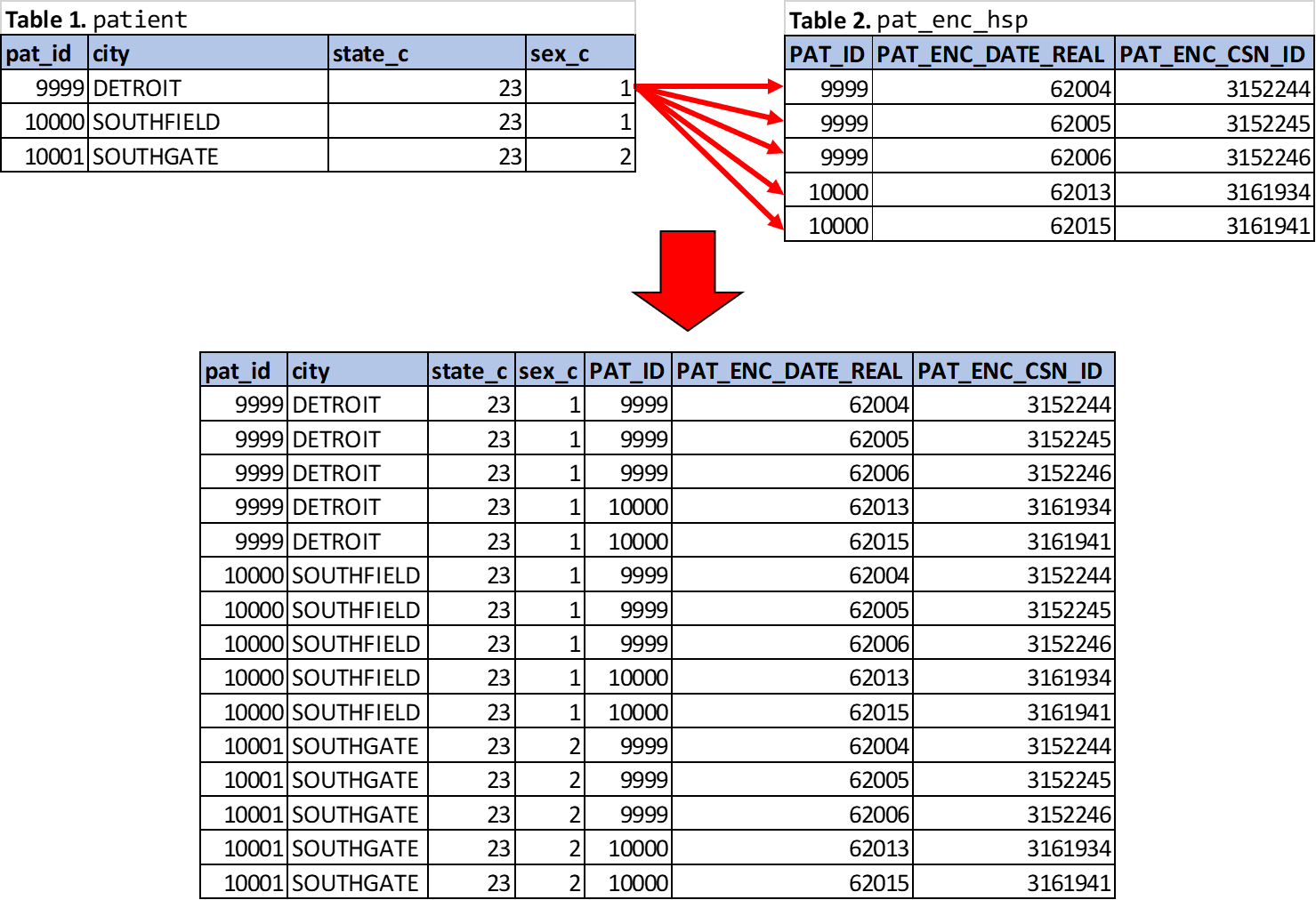
Figure 4.3: Cross Product (CROSS JOIN) of Table 1 and Table 2.
Practical Example
A possible use case for CROSS JOIN operations is taking a single set of values (e.g., serum creatinine) within a certain grouping (e.g., patients or hospital encounters) and performing a self-comparison within all values to identify changes meeting a specific definition. Some good applications of this technique are for helping to identify patients with acute kidney injury (AKI) or significant hemoglobin changes. As an example, below is a simple query where a single results table (let’s call it results) undergoes a CROSS JOIN operation against itself (yes, multiple instances of the same table can be used in the same query — in fact it is a very useful technique).
SELECT
  rslts.pat_id,
  rslts.pat_enc_csn_id,
  rslts.creatinine,
  rslts.creatinine_dttm,
  rslts_2.creatinine,
  rslts_2.creatinine_dttm,
  rslts_2.creatinine - rslts.creatinine AS scr_difference
FROM results AS rslts
  CROSS JOIN results AS rslts_2
WHERE
  rslts.pat_id = rslts_2.pat_id AND
  rslts.creatinine_dttm <> rslts_2.creatinine_dttm
The results from the above query are shown in Figure 4.4. The table product is all within-patient comparisons of the patient’s serum creatinine values, which can be used for determining whether any significant changes occurred (e.g., increases of ≥ 0.5 mg/dL). Note the WHERE clause in this query which contains two predicates to ensure that: i.) source and joined table rows are not cross-joined between patients (imagine cross-joining an entire 10,000-row-table against itself!); and ii.) results for the same date-time (within patients only thanks the first WHERE predicate) are not resulted (since the difference would be a constant — i.e., zero — which is unlikely to be useful for this specific example).
Full disclosure: the WHERE predicates nullify the ultimate effect of the CROSS JOIN since there is no longer a pure cross-product of the two input tables (i.e., the table product doesn’t have n x m rows). However, thinking through this example should help solidify the logical process by which SQL performs JOIN operations, which is a cross product followed by subsequent operations depending on the join type. As we’ll see in the OUTER JOIN subsection, a cross join can serve as a simpler, more efficient alternative (syntactically and computationally) to a LEFT JOIN for some situations.
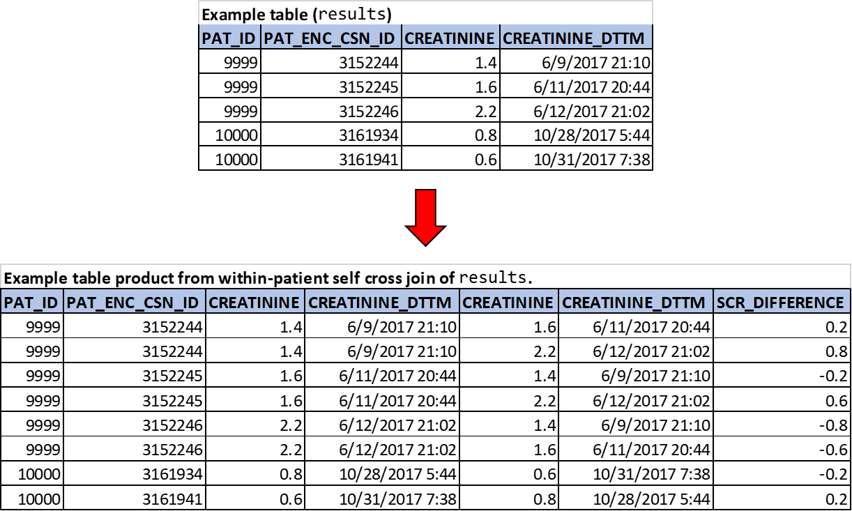
Figure 4.4: Practical example of CROSS JOIN: within-patient changes in serum creatinine values.
4.3 ON Subclause
As previously alluded to, the CROSS JOIN does not include the ON subclause given it’s a simple cross-table product. However, the INNER JOIN and OUTER JOIN do include the ON subclause, which is where join conditions are specified. Join conditions are simply logical predicates (we covered predicates when discussing WHERE clauses) which can take different forms in establishing the rules for joining two tables. There are two common designations to categorizing types of join conditions: equi-joins vs. non-equi-joins and simple joins vs. composite joins. The different approaches are not necessarily mutually exclusive.
Equi-joins are join conditions where equality is required between common key column values in the left and right tables (i.e., the join condition uses a = operator). Non-equi joins use alternate comparison operators or other types of operators such as logical or string (e.g., >, >=, <>, BETWEEN, LIKE). Ultimately, equi-joins and non-equi-joins both use comparative logic.
For the other categorization scheme, simple joins have a single predicate for their join conditions. Composite joins, on the other hand, have more than one join condition (each separated by an AND or an OR boolean operator). If you recall from Uniqueness: Candidate Key or Minimal Superkey in the last chapter, there may be tables whose primary key is a composite key — such tables may require a composite join depending on the circumstances. Below we’ll go through examples covering each of the different types of join conditions.
4.4 INNER JOIN
Takes a source (aka, left) table and right (aka, destination) table and produces a table product that includes only those rows which meet the join conditions specified in the ON subclause. INNER JOIN behaviors can create table products that — in relation to the left table — result in the removal of rows, no changes to the number of rows, or the addition of rows.
Theoretical Example
As alluded to in the definition, an INNER JOIN is a filtering join: any rows not meeting the join condition in the ON subclause are excluded. But this doesn’t mean the table product will necessarily be smaller, depending on the join conditions and the cardinality of the join (we’ll discuss join cardinality later in the next chapter).
INNER JOIN syntax and the CROSS JOIN syntax are the easiest to visualize and understand. See example query below demonstrating syntax for the INNER JOIN with source rows from the tables in Figure 4.2.
SELECT
  pats.pat_id,
  pats.city,
  pats.state_c,
  pats.sex_c,
  encs.pat_id,
  encs.pat_enc_date_real,
  encs.pat_enc_csn_id
FROM patient AS pats
  INNER JOIN pat_enc_hsp AS encs
    ON pats.pat_id = encs.pat_id
The input/output from the above query is shown below in Figure 4.5. In addition to specifying the JOIN type, the ON subclause is necessary to establish the join conditions, which are filtering conditions since we’re talking about an INNER JOIN. Using our example query and the visualized process shown in Figure 4.5, a useful basic language description to think of when interpreting SQL INNER JOIN syntax goes like this:
ON: “when the patient ID column from the destination/right table (pat_enc_hsp) matches the patient ID column from the source/left table (patient)…”INNER JOIN: “…link the matched rows so that any columns from the right table are made available to subsequent joins and query phases (signified by red arrows in Figure 4.5)…”- (implied) “…otherwise, do not include the source rows (i.e., from the left table) in the final table product (signified by black arrow and grayed out row from the final table product in Figure 4.5).”
Effectively, the above query example is resulting only those patients from Table 1 in Figure 4.2 that have encounters. As mentioned in the third step of the basic language description above, rows without a common pat_id (including if there are no matched rows in the right table, pat_enc_hsp) will be excluded from the final table product, as demonstrated with patient 10001.
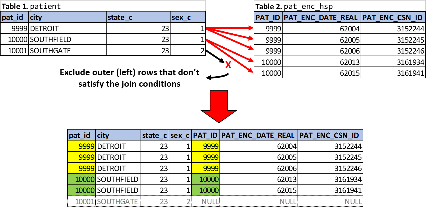
Figure 4.5: INNER JOIN of Table 1 and Table 2 on pat_id.
SQL logical processing actually evaluates the ON subclause before the INNER JOIN subclause. This may seem confusing when reading the syntax more like natural language, but makes sense when really considering what the join operation is actually doing: a conditional function cannot produce a result without first evaluating its arguments. Therefore, a join cannot be determined if its join conditions are not evaluated first. Like any high-level language (especially a declarative one like SQL), its syntax is meant to be more human-readable. The ON/JOIN syntax is a perfect example — the JOIN subclause is written before the ON subclause, similar to how more active sentence structures are generally preferred in the English language, notwithstanding the need to vary sentence structure sometimes for flow (e.g., “Joins occur if the join conditions are met” would often be preferred over “If the join conditions are met the joins occur”).
4.4.0.1 INNER JOIN vs. WHERE clause: What’s the Difference?
Hopefully, you’re asking yourself, If inner joins are filtering joins, then what’s the purpose of the WHERE clause? Strictly speaking, for simple multi-table queries with a predicate contained in the ON subclause of an INNER JOIN versus a WHERE predicate, there is generally no discernible difference between an INNER JOIN and a WHERE clause. However, for cases where users want “soft” filtering — as opposed to the absolute or “hard” filter of an INNER JOIN — combining LEFT (OUTER) JOINS and WHERE predicates will often allow more nuanced solutions, which we’ll cover in the LEFT OUTER JOIN section.
There may be query performance differences in favor of WHERE predicates when there are more JOIN operations occurring. Some users may also prefer INNER JOINS for code readability, particularly when there are filtering conditions distributed across many tables from multiple INNER JOINS. Although this approach allows the user to explicitly be aware of any filtering conditions at the point of the table join, not later in the WHERE clause, it is strictly a preference and not a requirement or convention.
Practical Example
Given the global utility of filtering, INNER JOINS have a breadth of use cases. Below is an example that combines equi-joins and non-equi-joins, as well as simple and composite joins.
SELECT
  ords.order_med_id,
  ords.description,
  deps.department_name
FROM order_med AS ords
  INNER JOIN clarity_medication AS meds
    ON ords.medication_id = meds.medication_id AND
       meds.pharm_subclass_c = 13 AND
       ords.ordering_date BETWEEN '20200101' AND '20200131'
  INNER JOIN clarity_dep AS deps
    ON ords.pat_loc_id = deps.department_id AND
       deps.rev_loc_id = 104001
The query results all basic medication orders (e.g., excludes non-premade admixtures) that were placed during January 2020 for a third-generation cephalosporin at West Bloomfield hospital. The same results could be obtained by changing from an INNER JOIN to a LEFT JOIN and moving the meds.pharm_subclass_c, ords.ordering_date, and deps.rev_loc_id predicates to the WHERE clause. Incidentally, the join type doesn’t have to be changed, since the remaining join conditions contain foreign keys (medication_id and department_id) that happen to never be missing in their respective right tables for these join scenarios. But as we’ll discuss under the Join Cardinality section in the next chapter, part of evaluating the database schema is understanding whether the tables have forced or optional participation for a join. It just so happens that clarity_medication.medication_id and clarity_dep.department_id are guaranteed to be present — if not, the INNER JOIN could filter out the source rows, as demonstrated in the theoretical example we discussed where patients without encounter information were removed from the query results.
It is good practice to only use INNER JOINS with the intent of doing so as a filtering join, that way the join type signals to the user how the join is meant to function (even if it’s the user’s own code). If the INNER JOIN is a simple equi-join that only includes required (not optional) foreign key columns you should probably change the join type to a LEFT (OUTER) JOIN, since the data is guaranteed to never be missing and thus no rows would ever be excluded. (That point may require some unpacking but is hopefully clearer after we discuss LEFT OUTER JOINS in the next section and [Join Cardinality].) Relatedly, the foreign key predicates (medication_id and department_id) could also be moved to the WHERE clause and provide the identical result. In fact, prior to ANSI SQL 92 the inner join conditions were specified like this in the WHERE clause; however, the modern “infixed” join syntax is preferred since the older syntax can be more difficult to interpret and can be more error prone.
This query also contains a few instances where understanding of schema and data definitions are required for proper query design. Any time an INNER JOIN condition points to a column that is missing systematically (i.e., missing not at random), the user needs to be aware in case the consequences are significant for their project. For example, the query was described as containing only “basic medication orders” which “excludes non-premade admixtures.” The reason for this systematic exclusion is because the meds.pharm_subclass_c data is always missing for non-premade admixtures — and any predicate within an INNER JOIN or WHERE clause that evaluates to false (or unknown in the case of null values) will result in excluded rows. Specifically, the order_med table contains one row per order and thus will always contain the “basic medication record.” Mixtures on the other hand contain multiple ingredients; therefore, meds.pharm_subclass_c data for each component cannot be obtained from a single medication_id — obtaining that data requires either the order_disp_meds or rx_med_mix_compon table depending on the situation, which will be covered during some exercises later in this manual.
Similarly, the meds.pharm_subclass_c and deps.rev_loc_id columns utilize category codes, which would require knowing how to investigate and select them (otherwise, how would you know that pharm_subclass_c = 13 means third-generation cephalosporins and that deps.rev_loc_id = 104001 means West Bloomfield hospital?). Later in this manual there will be exercises involving case scenarios that teach practical schematic knowledge and data definitions.
4.5 LEFT OUTER JOIN
Takes a source (aka, left) table and joined (aka, right or destination) table and produces a table product that includes all source rows — regardless if the join conditions specified in the ON subclause are satisfied — plus any joined table rows that meet the join conditions specified in the ON subclause. LEFT JOIN behaviors can create table products that — in relation to the left table — result in no changes to the numbers of rows or the addition of rows.
The LEFT OUTER JOIN (abbreviated SQL syntax of LEFT JOIN) is the default OUTER JOIN discussed throughout this manual. For completeness, the other OUTER JOINS are the RIGHT OUTER JOIN (abbreviated SQL syntax RIGHT JOIN) and FULL OUTER JOIN (abbreviated SQL syntax FULL JOIN), but will not be discussed given their uncommon use.
Theoretical Example
As alluded to in the definition, a LEFT OUTER JOIN (referred to hereafter as a LEFT JOIN) is a preserving join: all source rows are automatically preserved (unlike an INNER JOIN) in addition to any right table rows satisfying the join conditions (similar to an INNER JOIN). But unlike an INNER JOIN, for rows where the join conditions are not satisfied, columns from the right table rows (or non-preserved rows) will have NULL values added as placeholders to maintain the table structure; and the duplicate NULL rows from the non-preserved table are removed (i.e., each preserved row only appears once if there are no right table matches). This means the table product will contain at least as many rows as the left table and potentially more depending if any table rows satisfy the join conditions. Such knowledge coupled with schematic understanding of the query’s joins will help specify the DBI’s expectations for the query results. To demonstrate the LEFT (OUTER) JOIN syntax, see example query below with source rows from the tables in Figure 4.2.
SELECT
  pats.pat_id,
  pats.city,
  pats.state_c,
  pats.sex_c,
  encs.pat_id,
  encs.pat_enc_date_real,
  encs.pat_enc_csn_id
FROM patient AS pats
  LEFT JOIN pat_enc_hsp AS encs
    ON pats.pat_id = encs.pat_id
The input/output from the above query is shown below in Figure 4.6. The syntax is nearly identical to the theoretical example query for the INNER JOIN with the exception of the JOIN subclause. Similar to the INNER JOIN example, below is a basic language description of SQL LEFT JOIN syntax using our example query and the visualized process shown in Figure 4.6:
ON: “when the patient ID column from the destination/right table (pat_enc_hsp) matches the patient ID column from the source/left table (patient)…”LEFT JOIN: “…link the matched rows so that any columns from the right table are made available to subsequent joins and query phases (signified by red arrows in Figure 4.6)…”- (implied) “…otherwise, add back the source rows (i.e., from the left table) and use NULL placeholder values for the right table columns in the final table product, making sure to represent each NULL row from the non-preserved side only once (signified by black-to-red arrow in Figure 4.6).”
Effectively, the above query example is simply resulting all patients from Table 1 in Figure 4.2 and any encounter information if it’s available. If there are multiple encounter rows for a patient, their patient data will be repeated for that number of matched rows. As mentioned in the third step of the basic language description above, rows without a common pat_id (including if there are no matched rows in the right table, pat_enc_hsp) will be included in the final table product with their original source rows represented once and NULL placeholder values for each source row on the non-preserved side, as demonstrated with patient 10001.
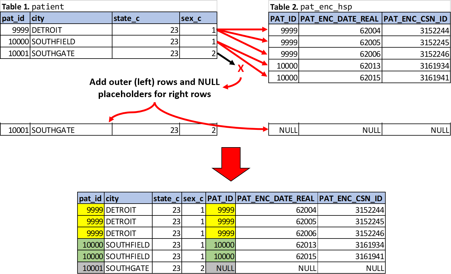
Figure 4.6: LEFT JOIN of Table 1 and Table 2 on pat_id.
Practical Example
LEFT JOINs are by far the most common SQL join operation. One reason is because filtering operations don’t require an INNER JOIN and can be done with a combination of LEFT JOINs and WHERE predicates; and many users elect to take this approach, at least for simpler queries. But there are operations that would otherwise be much more difficult without the LEFT JOIN. Yet, despite their ubiquity LEFT JOINs can also be the most difficult join type for beginner DBIs to fully take advantage of in practice. LEFT JOINs allow much potential for nuance in obtaining desired query results. Take the following query below as an example.
DECLARE @start DATETIME = '20200301 00:00:00.000'
DECLARE @end DATETIME = '20200331 23:59:00.000'
SELECT DISTINCT
  encs.pat_enc_csn_id,
  CAST(encs.hosp_admsn_time AS DATE) AS admsn_date,
  CAST(encs.hosp_disch_time AS DATE) AS disch_date,
  DATEDIFF(DAY,
           CAST(encs.hosp_admsn_time AS DATE),
           CAST(encs.hosp_disch_time AS DATE)) + 1
    AS los_days,
  IIF(ords.pat_enc_csn_id IS NOT NULL,
      1,
      0) AS cefepime_ordered_on_P2
FROM pat_enc_hsp AS encs
  LEFT JOIN clarity_adt AS adts
    ON encs.pat_enc_csn_id = adts.pat_enc_csn_id
  LEFT JOIN order_med AS ords
    ON encs.pat_enc_csn_id = ords.pat_enc_csn_id AND
       ords.description LIKE 'cefepime%' AND
       ords.pat_loc_id = 1010010023
WHERE
  adts.department_id = 1010010023 AND
  encs.adt_pat_class_c = 101 AND
  (
    (encs.hosp_admsn_time BETWEEN @start AND @end OR
     encs.hosp_disch_time BETWEEN @start AND @end) OR
    (encs.hosp_admsn_time < @start AND
     encs.hosp_disch_time > @end)
  )
4.5.0.1 What Data the Query is Pulling: Role of the LEFT JOIN
The query pulls all inpatient encounters in the P2 patient care unit at Henry Ford Detroit Hospital for patients hospitalized any time in March 2020. Although the LEFT JOIN conditions include requirements for cefepime orders associated with the P2 patient care department (i.e., pat_loc_id = 1010010023), notice that the description of our query pull didn’t mention them as a requirement — predicates from the WHERE clause were reflected in our description. Remember, with LEFT JOINs all source rows are preserved and all rows from the right table (i.e., the non-preserved side of the join) that don’t fulfill the join conditions will have their columns tagged with NULL placeholders and be represented only once. The point of this explanation is to highlight the “soft” filtering performed by the LEFT JOIN and that it doesn’t determine your result set (as opposed to the WHERE clause which includes only those rows satisfying the predicate search conditions). As such, LEFT JOINs are most commonly used when join conditions are guaranteed (e.g., ON subclause includes a required foreign key; right table is a user-created table without missing data); or in situations where we don’t want commit the entire result set to some filtering conditions but want visibility into missing data. Understanding missing data is not only valuable for the self-obvious reason, but also because it can be used to create new columns (variables), as we’ll see in the Using LEFT JOIN Conditions to Create New Column section.
The LEFT JOIN with order_med will simply carry forward all source rows from pat_enc_hsp to the next logical processing phase (the WHERE clause). All joined rows will be included and non-preserved rows will be represented once with NULL column placeholders. To help us visualize what’s happening with this LEFT JOIN prior to the WHERE clause, let’s examine some hypothetical joined and non-preserved rows from this query, as shown in Figure 4.7 below. For simplicity we’ll include only those columns participating in the ON subclause, respectively (encs.pat_enc_csn_id, ords.pat_enc_csn_id, ords.description, and ords.pat_loc_id).
.png)
Figure 4.7: Theoretical source rows from order_med LEFT JOIN.
For the LEFT JOIN in this query there are three join conditions that are dictating the interim row results in Figure 4.7. Expressed in natural language, our LEFT JOIN is conditional upon orders placed during the index encounter for cefepime that are associated with the P2 patient care department (i.e., pat_loc_id = 1010010023). For rows where any of these conditions are not met the LEFT JOIN will preserve the source rows and include NULL placeholders for any non-preserved row columns (ords.pat_enc_csn_id, ords.description, and ords.pat_loc_id), as shown with pat_enc_csn_id 10000986411, 10000084504, and 10001630152. It is important to note that our pat_enc_csn_id equality condition guarantees that for each encounter there will be one row (with NULL ords.pat_enc_csn_id value) or at least one row (with non-NULL ords.pat_enc_csn_id value or repeating values if there are more than one row meeting all join conditions). We’ll revisit this point towards the end of this discussion.
Conversely, for each row where all join conditions are met the joined rows will be displayed in addition to the source row, as shown with pat_enc_csn_id 10000000000 and 10007377149. A notable case is pat_enc_csn_id 10000000000, since there are duplicate rows displayed as a result of four total rows in order_med that satisfied the join conditions. If we would have included ords.order_med_id in our example output we would have seen four unique order_med_id’s since that is a primary key for the order_med table (the relevance of avoiding these unique values will come to bear). We’re early in the logical processing of this query; so, the DISTINCT clause hasn’t had the opportunity to remove duplicates, and any duplication from our LEFT JOIN will be carried forward to the next processing phase. As a reminder, the interim rows in Figure 4.7 are for example; realistically, all columns from pat_enc_hsp and order_med would be available to the WHERE clause.
4.5.0.2 Using LEFT JOIN Conditions to Create New Column
Skipping ahead to the SELECT and DISTINCT clauses, it is important to highlight how the LEFT JOIN is helping support an analytic purpose in this query. The cefepime_ordered_on_P2 expression is using the IIF() function whose output is dichotomous — specified to be binary in this case — which indicates if there was a P2 cefepime order during the encounter. (IIF() is a SQL language extension and is a shorthand version of a CASE ... ELSE expression; which is a common way of using a list of conditions to create specific results.) Specifically, it is evaluating if ords.pat_enc_csn_id is not NULL; which we learned happens when all logical conditions have been satisfied. Therefore, we can interpret the presence of non-NULL ords.pat_enc_csn_id values as meaning there was a P2 cefepime order. But what about our duplicate rows for pat_enc_csn_id 10000000000? Since the only way that ords.pat_enc_csn_id duplicates can be produced in this example is through satisfying the join conditions, our cefepime_ordered_on_P2 expression is guaranteed to have a constant value of 1, which would be repeating for pat_enc_csn_id 1000000000. Similarly, NULL-valued ords.pat_enc_csn_id values are guaranteed to be a single row for each source row, which will also be a constant value of 0.
Lastly, after the SELECT clause, the DISTINCT clause will simply remove any duplicate rows, which addresses our previous discussion about constant values for cefepime_ordered_on_P2 — the final product will be guaranteed to yield either a 0 or a 1 value for each source row (encounter) in our code. Remember the point in the previous paragraph about what would happen if we included order_med_id? If those values were included we would have duplicate rows for some encounters (e.g., pat_enc_csn_id 10000000000), which would be undesirable if the analytic purpose for our example query was for each row to represent an encounter and whether there was a P2 order for cefepime. (Imagine tallying your results and counting encounters with duplicate rows multiple times — this would systematically overestimate the number of encounters with P2 orders for cefepime since NULL-valued data from the right tables cannot be duplicated by definition.)
4.5.0.3 An Aside: Datetime Search Conditions
A secondary but useful teaching point in our query example relates to the datetime-based predicates in the WHERE clause. For the previous basic language description of what our query was effectively doing, notice that it was described as patients hospitalized during March 2020; not admitted in March 2020, discharged in March 2020, or even admitted or discharged in March 2020. Refer to the first subgroup of temporal predicates from the WHERE clause (as shown below). They may seem like overkill, but filtering based on admission or discharge timing will overlook patients whose admission and discharge didn’t occur on the same month (which was the case for 17% of all HFHS inpatient encounters in 2020).
encs.hosp_admsn_time BETWEEN @start AND @end OR
encs.hosp_disch_time BETWEEN @start AND @end
Our other temporal predicates are shown below as well. Their logic includes patients who were in the hospital during March 2020 but whose admission and discharge occurred before and after March 2020, respectively. Less than 1% of HFHS inpatient encounters in 2020 were more than 30 days, so this logic is unlikely to impact our results. However, there’s an argument to be made for being comprehensive in your query logic, especially if there is no downside and it’s one less threat to be vigilant about when validating your results. (Plus, for the first case in particular we have empiric evidence to support the coding practice — I highly encourage you to gather this type of empiric data to inform your approach to query design.) Just in case you were wondering, our example query results in 185 rows (encounters): 13 encounters had a length of stay greater than 30 days, three of which were associated with P2 cefepime orders. Whether that is significant depends on the project; hence, my recommendation to adopt universal precautions when the return on investment makes sense. There is a simpler, more optimal way to achieve these same query results — it requires more schema knowledge and attention to detail, but will serve as a good example in later exercises.
encs.hosp_admsn_time < @start AND
encs.hosp_disch_time > @end
4.6 Clauses of the SELECT statement: A Multi-table Example
Now, similar to the approach taken in Basic Syntax (Single-table Query): Clauses and Language Elements, we will step through and analyze the multi-table query from Figure 4.1 with an emphasis on table JOIN operations.
As we previously established, in binding order (of logical query processing) we see there are five clauses/subclauses: 1. FROM, 2. ON/JOIN subclauses, 3. SELECT, 4. ORDER BY, and 5. TOP.
FROM clause
FROM pat_enc_hsp AS encsSpecifies the table name argument
pat_enc_hsp(assumes the database context has been specified as discussed in the section Microsoft SQL Server Management Studio (SSMS): Getting Started).ASkey word is optional for establishing table alias (note: aliases can also be established using the syntax<alias> = <expression>). User-specified table aliasencsis also optional. As mentioned in the FROM clause narrative in Basic Syntax (Single-table Query): Clauses and Language Elements for 2.1, table aliases become more important when creating multi-table queries for the sake of code readability. Refer to that discussion for more details about how to specify column names from unaliased tables.Data from the
pat_enc_hsptable are now available for manipulation and are presented for further processing to the next query phase, the ON/JOIN subclauses for our multi-table query example. (For single-tabe queries the WHERE clause would be the next logical processing phase.)ON/JOIN subclauses
This phase of the query includes both INNER and LEFT JOIN’s, so they will be discussed individually.
INNER JOIN
INNER JOIN order_med AS ords
  ON encs.pat_enc_csn_id = ords.pat_enc_csn_id AND
     encs.hospital_area_id = 101001 AND
     ords.ordering_mode_c = 2 AND
     ords.ordering_date BETWEEN @start AND @end AND
     ords.medication_id IN (180774, 501060)
The INNER JOIN for this query example is a composite join consisting of multiple join conditions, which can be broken up into two basic groups as shown below. Remember, INNER JOIN’s are filtering joins — all conditions must be met in order for the respective left table rows to be available for subsequent joins or later query phases.
Equi-join conditions:
encs.pat_enc_csn_id = ords.pat_enc_csn_idRequires that any source rows (encounters) from
encs(i.e.,pat_enc_hsp) must be present in the right table (i.e., the encounter must contain a medication order).encs.hospital_area_id = 101001Requires that the
hospital_area_idfrom the source row (encounter) be equal to101001, which corresponds to Henry Ford Hospital Detroit. Identifying that code requires some workflow and will be discussed in later examples.ords.ordering_mode_c = 2Requires that the order from the right table was placed with an
ordering_mode_cof2, which corresponds to inpatient ordering mode. Similar to thehospital_area_id, identifying the correct ordering mode code requires some workflow and will be discussed in later examples.
Non-equi-join conditions
ords.ordering_date BETWEEN @start AND @endRequires that order from the right table was placed between the
@startdate variable (July 1, 2019) and the@enddate variable (June 30, 2020).ords.medication_id IN (180774, 501060)Requires that medication from the order in the right table must have a
medication_idof either180774or501060, which corresponds to medication records for meropenem-vaborbactam. Identifying these codes will be discussed in later examples.
When considering a single logical processing phase SQL is executed as an all-at-once operation. For the above INNER JOIN, what that means is the order of the ON predicates doesn’t affect the final result. However, each JOIN subclause is executed in the order written.
LEFT JOIN
LEFT JOIN patient AS pats
  ON encs.pat_id = pats.pat_id
LEFT JOIN zc_med_unit AS unts
  ON ords.hv_dose_unit_c = unts.disp_qtyunit_c
LEFT JOIN ip_frequency AS frqs
  ON ords.hv_discr_freq_id = frqs.freq_id
The LEFT JOIN’s for this query example are all simple equi-joins. Remember, LEFT JOIN’s are preserving joins — source rows will be preserved regardless if the join conditions are met, albeit the output behavior will be different for the non-preserved side of the join (i.e., for the right table in each LEFT JOIN). However, as previously stated the joins are executed in the order written. This means the preceding INNER JOIN can impact rows from both
pat_enc_hspandorder_med, which both contribute source rows to the LEFT JOIN’s described above — if any rows from either of those tables were dropped due to not satisfying all INNER JOIN conditions they will not be available to these subsequent LEFT JOIN’s.WHERE clause
For the sake of illustrating INNER JOIN’s this query does not contain a WHERE clause. However, as discussed in the Inner Join section, there is no difference in query results between a predicate that is written into the join conditions (i.e., ON subclause) versus the search conditions (i.e., WHERE clause). As previously mentioned, while the results may be identical the SQL execution may be quicker when predicates are included in the WHERE clause. Some SQL practitioners may prefer predicates within INNER JOIN’s for code readability, that way the columns involved in predicates can be contextualized with their tables.
SELECT clause
Source rows not removed from the composite INNER JOIN are available for presentation or further manipulation. This query highlights a few different expression types, including simple expressions (column, function) and complex expressions. See Figure 4.1 for more details about the specific expression types. In keeping with the idea to introduce some practical SQL information along the way, we’ll briefly discuss the three functions,
CAST,DATEDIFF, andCONCAT, especially since theage_yrscolumn involves a nested function. The full documentation for these functions is available at Microsoft Transact-SQL Reference (Database Engine).SELECT pats.pat_mrn_id AS mrn, CAST(DATEDIFF(MONTH, pats.birth_date, encs.hosp_admsn_time) / 12. AS NUMERIC(4,1)) AS age_yrs, encs.pat_enc_csn_id AS encounter_id, ords.order_med_id AS order_id, ords.description AS medication, ords.hv_discrete_dose AS ordered_dose, unts.name AS ordered_dose_units, frqs.freq_name AS ordered_frequency, CONCAT(ords.hv_discrete_dose, ' ', unts.name, ' ', frqs.freq_name) AS ordered_regimen, ords.order_inst AS ordered_dttmCASTfunctionTransforms an expression from one data type to another. Data types is its own topic, but for beginning DBI’s there are two practical reasons for transforming data types: presentation purposes or requirements (or both). For the query example the reason is mostly for presentation, which will make sense after we unpack the
DATEDIFFfunction. See the Microsoft DATEDIFF documentation for more information.DATEDIFFfunctionTakes three arguments, a specified level of time precision (e.g., seconds, days, years) and begin and end boundaries, which are used to determine the interval. The function output is in the form of a signed integer.
Why didn’t the query just specify the desired interval to be in years instead of months divided by 12? To answer this question, let’s compare the output from the following two statements:
SELECT DATEDIFF(YEAR, '20210101', '20211231')versusSELECT DATEDIFF(YEAR, '20201231', '20210101'). After executing these statements, it’s clear that theDATEDIFFfunction uses thedatepartargument (YEARfor our example) to establish the boundary for determining a count, not necessarily calendar distance as one might intuitively expect. While the difference for this example is unlikely to be significant for adults, it does not fit the normal intent for determining age. For a more exact estimate of a patient’s age one could take a more precise time interval (e.g., days), but this would be arbitrarily inexact no matter which divisor we choose due to leap years. That leaves either weeks or months, both of which are reasonable options, although if we were being purists we’d use weeks since it’s more precise.Remember, the
DATEDIFFoutput is an integer, meaning we’re now left with one remaining question to address: do we want to perform integer division by 12 or decimal division by 12? If whole number precision (always rounding down) is acceptable then we could simplify ourage_yrscomplex function to beDATEDIFF(MONTH, pats.birth_date, encs.hosp_admsn_time) / 12. For the practical purposes of determining an adult’s age that would likely be sufficient. However, if we want to retain fractions of a year then we need to perform decimal division (this may make sense for other applications where the rounding factor is a relatively larger proportion of the final value).The concept of dividing an integer data type by a decimal data type requires us to briefly mention a concept in SQL called data type precedence, which refers to a hierarchy of data types. This hierarchy determines how different data types behave when they are combined using an operator, more specifically the implicit conversion of the lesser data type to the greater data type that takes place. For our example, that refers to the the
/used to divide ourDATEDIFFoutput by12.. Did you notice that the divisor in our example is12.and not12? The decimal data type has greater precedence than the integer data type (see Data Type Precedence for more information). This means that dividing an integer by a decimal will implicitly convert theDATEDIFFoutput to a decimal, and thus our final result will be a decimal data type to a default precision of six decimal places. So, if we truly desired ourage_yrscolumn to be a decimal it would be best to round our result for presentation purposes; hence, theCASTfunction that is wrapping theDATEDIFFfunction in our example.The moral of the story is… that date and time- based functions and data type precedence are complicated — be warned that unexpected behaviors may occur in your queries unless you have a stronger understanding of how these concepts affect your results. I highly recommend experimenting and seeing if you can predict the results when varying
DATEDIFFarguments or when working with complex expressions involving different data types. Simple SELECT statements using functions that only depend on scalar or variable expressions as arguments doesn’t require use of actual data tables and is a great way to experiment [this is how we comparedSELECT DATEDIFF(YEAR, '20210101', '20211231')andSELECT DATEDIFF(YEAR, '20201231', '20210101')].CONCATfunctionA string function that joins up to 254 string expressions into one final string result. (The same results can be achieved by using the
+operator with string values, although this can become a problem once numeric data types are included, which highlights the utility of theCONCATfunction.) TheCONCATfunction can serve multiple purposes, including combining a mixture of scalar and column expressions for a more descriptive, useful result such as theordered_regimenexpression in our example.
ORDER BY clause
Source rows presented from the SELECT clause are sorted according to the ORDER BY column(s) (either a specified column name, alias [if applicable], or integer corresponding to position number in the select list). Our query example is sorting by
mrnandordered_dttmaliases according to default setting of ascending order (descending order can be specified with use of key wordDESCafter the column name). The ORDER BY clause can sometimes be for presentation purposes; however, for our example it serves a filtering function essentially because of the TOP clause specified in the SELECT clause, which is discussed below.TOP clause
Limits the number of rows returned from the SELECT statement to the top 10 percent, as determined by the sort order of
mrnandordered_dttmcolumns. If the inclusion of ties is desired theWITH TIESkeyword is required after the integer arguments in the TOP clause.Query Results (de-identified through random noise added to all potential PHI)
%20with%20clauses%20&%20elements_results.png)
Figure 4.8: Results from Multi-table Query Example.