2 Basic Syntax (Single-table Query): Clauses and Language Elements

2.1 SELECT statement and Logical Processing Order

Querying is the act of selecting data from databases. The foundational SQL activity for querying is the SELECT statement, whose syntax includes the list of notable (but non-exhaustive) clauses below. Of note, SELECT statements also contain the SELECT clause; the difference being that the statement is the entire unit of SQL work (a query containing multiple clauses and language elements), whereas the clause is a single syntactical element. An important feature of SQL is that operations are not executed in the order written; rather, they are subject to the phases of logical processing order (aka, binding order). The binding order of SQL query processing phases are specified in the list below.

1. FROM
   1. ON (specified in the FROM syntax)
   2. JOIN (specified in the FROM syntax)
2. WHERE
3. GROUP BY
4. HAVING
5. SELECT
   1. DISTINCT (specified in the SELECT clause syntax)
6. ORDER BY
7. TOP (specified with arguments in the SELECT clause syntax)

It may not make sense at first, but considering that the original intent for SQL was to read more like written English, it begins to make sense. For example, before selecting data (i.e., the SELECT clause) once must first point to the source (i.e., FROM clause and ON/JOIN subclauses). Back-end SQL implementation (i.e., physical query processing by the optimizer) does not always follow these rules for the sake of optimization, so long as the ultimate result is not affected. The important point is that each clause is only capable of processing information presented to it by the preceding query phase. Conceptually following the flow of intermediate results within a query is essential to understanding the expected results, producing the desired results, and troubleshooting unexpected results. Multiple examples in this manual will conceptualize intermediate table results — which are normally invisible to the user — to give the reader a better idea of the data manipulations occurring within the SELECT statement.

2.2 Clauses of the SELECT statement: A Basic Example

To demonstrate the basic syntax of a SELECT statement and the conceptual flow of intermediate query results according to logical processing order, let us examine the query example below in Figure 2.1.

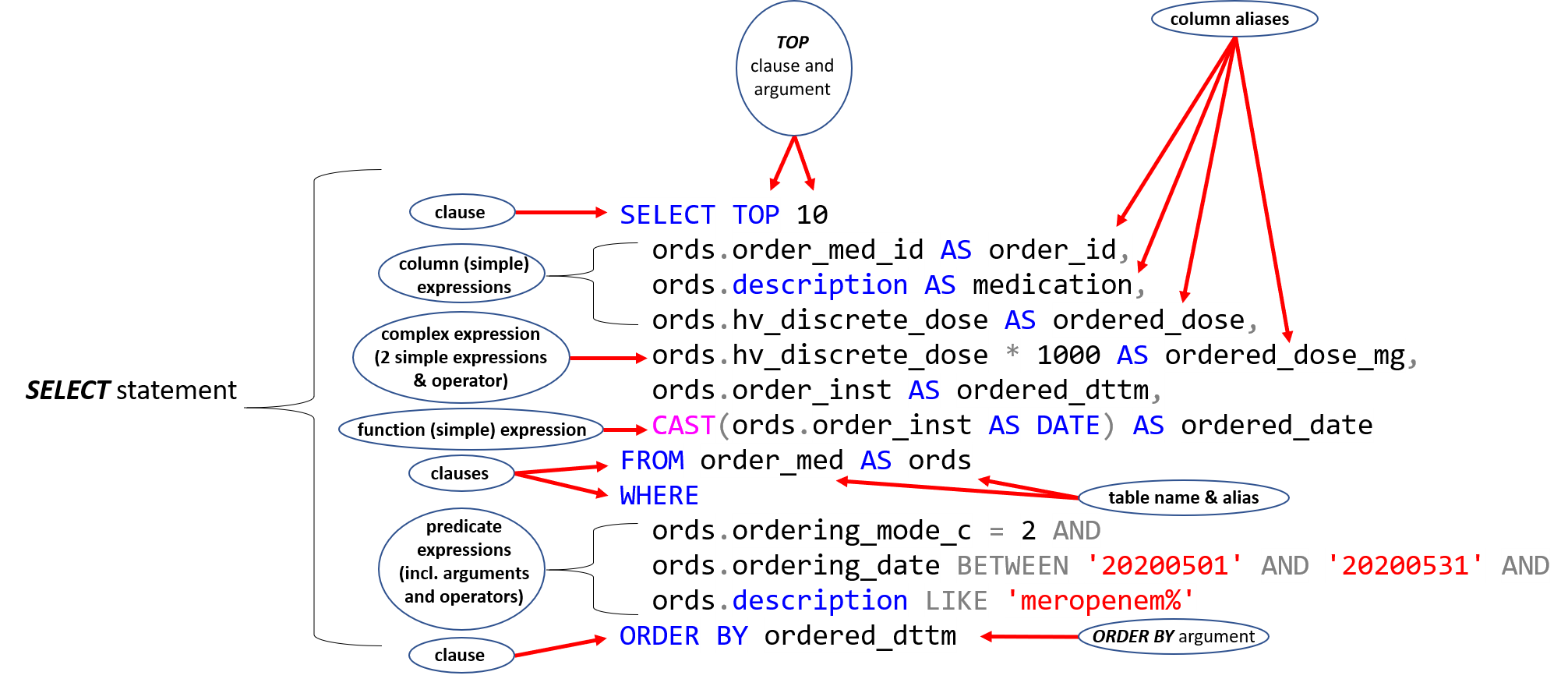
Figure 2.1: Basic Query Example.

Dissecting Figure 2.1 in order of logical processing, we see there are five clauses: 1. FROM, 2. WHERE, 3. SELECT, 4. ORDER BY, and 5. TOP. Before delving too deeply into the other language elements, let’s use a plain language description of these clauses and their syntax. SSMS output from the query in Figure 2.1 is shown in Figure 2.2 at the bottom of this page.

1. FROM clause

   FROM order_med AS ords

   Specifies the table name argument order_med (assumes the database context has been specified as discussed in the section Microsoft SQL Server Management Studio (SSMS): Getting Started).

   AS key word is optional for establishing table alias but is preferred by some since it provides clearer, more literate code. (Note: aliases can also be established using the syntax <alias> = <expression>). User-specified table alias ords is also optional in this example (generally done for subsequent referencing and code readability — this point becomes more important once we progress to multi-table queries).

   If table aliases are not used there would be two other options when specifying columns names:

   1. The entire qualified <table name>.<column name> could be specified. For example, if order_med wasn’t aliased the SELECT columns in Figure 2.1 would have the ords replaced by order_med.
   2. No alias or table name is used when specifying the column. This works for single-table queries since there are no other tables. If there were other tables there would be the possibility of an ambiguous reference error (e.g., if two tables contained the same column name the query would be non-deterministic).

   Data from the order_med table are now available for manipulation and are presented for further processing to the next query phase, the WHERE clause for this example. (Note: for multi-table queries, the next query phase would be the ON/JOIN phases.)

2. WHERE clause

   WHERE
     ords.ordering_mode_c = 2 AND
     ords.ordering_date BETWEEN '20200501' AND '20200531' AND
     ords.description LIKE 'meropenem%'

   Source rows are presented from the previous query phase result set (FROM clause). Remember, this is the conceptual, not physical flow of data and is not visible to the SQL user. Each row of the available intermediate data thus far is evaluated against each predicate expression from the search condition. Only those rows for which all predicates evaluate to TRUE are presented to the next query phase.

   For Figure 2.1, only rows from order_med with an inpatient ordering mode, an ordering date in May 2020, and an order description that starts with “meropenem” (which could potentially include meropenem-vaborbactam), are presented to the next query phase (SELECT clause).

3. SELECT clause

   SELECT
     ords.order_med_id AS order_id,
     ords.description AS medication,
     ords.hv_discrete_dose AS ordered_dose,
     ords.hv_discrete_dose * 1000 AS ordered_dose_mg,
     ords.order_inst AS ordered_dttm,
     CAST(ords.order_inst AS DATE) AS ordered_date

   Source rows are presented from the previous query phase result set (WHERE clause). One last reminder, this is the conceptual, not physical flow of data and is not visible to the SQL user.

   Elements from the SELECT clause (the select list) are presented to the next query phase (TOP clause). The select list consists of expressions, which can take many forms, and is discussed in SQL Language Elements: A Basic Example Continued.

4. ORDER BY clause

   ORDER BY ordered_dttm

   Source rows are presented from the previous query phase result set (SELECT clause) and sorted based on the argument(s) (column or column number) specified in the ORDER BY clause. Remember, since column aliases were established in the SELECT phase (i.e., earlier in the logical order), they can be referenced starting in the ORDER BY clause.

   Given the ORDER BY syntax, ords.order_inst, ordered_dttm, or 5 would be equivalent for the query example and result in the query set being sorted by ords.order_inst (in ascending order by default; or descending order if the ORDER BY argument — ordered_dttm in Figure 2.1 — is followed by DESC). The argument 5 is equivalent because it’s the fifth column from our select list.

   This query phase is mostly for display purposes or to limit the return rows (when used in conjunction with the TOP clause, as shown in the next query phase section). Sorted query results are presented to the next query phase (TOP clause).

5. TOP clause

   TOP 10

   Source rows from the previous query phase (ORDER BY clause) are presented to the TOP clause, which is specified by the argument 10, indicating that only an ordered subset of 10 rows will be returned. For the query in Figure 2.1, the TOP clause has the effect of selecting the first 10 inpatient meropenem-like orders in May 2020. I use the term “meropenem-like” since, as pointed out in the WHERE clause explanation, the example query could have resulted orders for meropenem-vaborbactam if they would have occurred after 2020-05-01 00:00:00.000 and before 2020-05-02 16:34:00.000. We will discuss approaches later for selecting reliable search conditions in the WHERE clause.

6. Query Results

   SSMS output from the query in Figure 2.1 is shown in Figure 2.2 below.

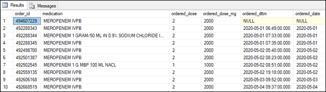
Figure 2.2: Results from Basic Query Example.

2.3 SQL Language Elements: A Basic Example Continued

Now that we have established a basic understanding of the data manipulation occurring within some common clauses of the SELECT statement, let us introduce some important language elements from the query example in Figure 2.1: expressions, predicates, operators, and column/table aliases.

2.3.1 Expressions

Combination of symbols and operators that evaluates to a single value when the expression is evaluated individually for each row in the result set.

This definition may seem abstruse to the beginning SQL practitioner — how could an expression in the SELECT list evaluate to more than one value? The answer: subquery expressions. Take the following example using a made-up table #nmbrs which includes the column digit whose arbitrary domain is the integers 0 through 5. (Focus on the SELECT statement; this example happens to introduce some preceding syntax which is new and will be covered later with more advanced materials.)

SET NOCOUNT ON 
DROP TABLE IF EXISTS #nmbrs 
CREATE TABLE #nmbrs (digit INT)
INSERT INTO #nmbrs (digit)
VALUES (0), (1), (2), (3), (4), (5)

SELECT 
  digit,
  (SELECT TOP 1 digit FROM #nmbrs) AS subquery_output
FROM #nmbrs    

See the output below in Figure 2.3. The subquery is a valid expression since the TOP clause has an argument of 1 and thus evaluates to a single value — this would not be the case if the TOP clause argument was greater than 1. This example is to simply illustrate the definition of an expression while stippling some other concepts along the way that will eventually become important (e.g., CREATE TABLE syntax, subquery expressions).

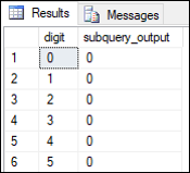
Figure 2.3: Query output with valid subquery expression.

As indicated in Figure 2.1, the SELECT phase (clause) contains both simple expressions (single element) and complex expressions (≥ 2 elements connected by ≥ 1 operator).

2.3.1.1 Simple expressions (single element)

• Column expression is the most common example of a simple expression (4 of the 6 columns in the example query are column expressions). They are simply the inclusion of a properly qualified column name (including aliases) in the SELECT list.
• Function expression is a function as an expression. Many functions take multiple arguments/inputs, but are still considered as a single element (i.e., a simple expression). The ordered_date variable is a simple function expression which uses the CAST function to transform ordered_dttm from a datetime to a date variable. Specifically, it uses the simple expression ords.order_inst and a data_type argument (AS DATE) to produce its result. Data types will be covered in more detail later.
• Constant expression (aka, scalars, literals) is a simple expression with a constant value. It isn’t utilized in Figure 2.1, but a simple practical example would be 'pre' AS study_period, which could populate a theoretical new column entitled constant_variable with every row having a value of pre. Use cases for constant expressions will be discussed further, but are often used as placeholders in a SELECT statement.
  • Note: SQL requires surrounding single quotes ['<string>'] to delimit (i.e., specify explicit begin and end boundaries for) character strings, otherwise SQL does not have clear instructions on how to parse the potential character strings it encounters. For example, from our constant expression example with the single quotes removed (pre AS study_period) is the variable name pre or pre AS study_period ?.
• Variable expression is a user-defined variable that assumes a constant value and can be called within the clauses of a SELECT statement. For example, a variable could be established for a begin date of interest which is later referenced in a WHERE predicate. This topic will be covered in later sections since it introduces new syntax.

2.3.1.2 Complex expressions (≥ 2 elements connected by ≥ 1 operator)

• The column ordered_dose_mg is a complex expression consisting of a column expression (ords.hv_discrete_dose), an arithmetic operator (*), and a scalar expression (1000). The end result is multiplying ords.hv_discrete_dose by 1000 in order to express ords.hv_discrete_dose in milligrams instead of grams. Of course, this logic will only produce the desired result if ords.hv_discrete_dose is always expressed in grams. Hint: some meropenem medication records express hv_discrete_dose in grams and some in milligrams — this is likely an unintended discrepancy but a great example of using proper exploratory data analysis and/or schematic data knowledge to inform the proper creation or transformation of a variable.

2.3.2 Predicates

An expression that evaluates to TRUE, FALSE, or UNKNOWN (i.e., trinary logic).

Some may be familiar with the concept of Boolean logic which evaluates binarily, i.e., TRUE/FALSE. However, the concept of nullability is somewhat unique to the SQL dialect and results in a three-pronged (trinary) logic. As an example in Boolean logic, if a = 1 then a > 0 is obviously true; a < 0 is obviously false. But what if a is missing or a = carrot? Binary logic would dictate that if a is missing or is a character string value (e.g., carrot) then a > 0 is false: the expression definitely is not true (in binary terms). However, in trinary logic those same statements are not necessarily true or false since the predicate cannot be evaluated. In the simplest terms, a NULL value is treated as an unknown value: it arises from inapplicable, miscellaneous, missing, or unknown data values. Using a NULL-valued variable a, NULL values tend to either propagate NULL values if present in an expression (e.g., 1 + a) or result in omitted rows (e.g., WHERE a < 0). See Example 2.1 below for another simple illustration of trinary logic.

Example 2.1 (Demonstration of Trinary Logic.) Let us assume that the predicate expression is \(a + b > 2\), where \(a\) and \(b\) are table columns containing numeric data.

Predicate 1:

a = 1, b = 0

\(a + b = 1\)

→ Evaluates to FALSE

Predicate 2:

a = 1, b = NULL

\(a + b = NULL\)

→ Evaluates to UNKNOWN

Predicate 3:

a = 1, b = 2

\(a + b = 3\)

→ Evaluates to TRUE

Predicates can be present in multiple query phases (e.g., ON/JOIN, WHERE, and SELECT). For Figure 2.1, the WHERE phase contains predicate expressions separated by AND operators and take the format of column expression + operator + argument(s):

1. The first predicate expression ords.ordering_mode_c = 2 contains ords.ordering_mode_c (column expression), = (comparison operator), and 1000 (a scalar expression argument).
2. The second predicate expression contains ords.ordering_date (column expression), BETWEEN (logical operator), and '20200501' AND '20200531' (complex expression argument consisting of two scalar expressions and a logical operator).
3. And lastly, the third predicate expression ords.description LIKE 'meropenem%' contains ords.description (column expression, which for this predicate is the match expression within the LIKE syntax), LIKE (logical operator), and 'meropenem%' (scalar expression with the wildcard string operator, %). The various data types in these predicates’ arguments (exact numeric, date and time, character string) will be covered in more detail later.

Predicates are evaluated against each row of intermediate data from the previous query phase (the FROM clause for our query example in Figure 2.1). The intermediate data being presented to the WHERE clause will contain many data rows from order_med that are unfamiliar since they logically preceded the ultimate results displayed to us in Figure 2.2. A glimpse into those pre-WHERE clause data will help to illustrate the effect of our predicate expressions. See Figure 2.4 below for a theoretical sample of intermediate table results being presented to the WHERE clause from our query example in Figure 2.1. Stepping through the predicate expressions for each row from our theoretical sample data yields the following results:

• Based on the example data in Figure 2.4, all rows would evaluate as TRUE against the first predicate from Figure 2.1 (ords.ordering_mode_c = 2);
• Rows 1, 6, and 9–10 would evaluate as TRUE against the third predicate (ords.description LIKE 'meropenem%');
• All rows would evaluate as FALSE against the second predicate (ords.ordering_date BETWEEN '20200501' AND '20200531').
• Ultimately, all predicates must evaluate as TRUE for a given row of source data to be presented after the WHERE phase. If the example data in Figure 2.4 were the actual source rows presented to the WHERE clause in Figure 2.1, no rows would be presented to the SELECT phase. Predicate expressions evaluated against rows whose participant column expressions contain NULL values would be excluded. No such rows exist in Figure 2.4, but an example would be if a row contained a NULL value for ordering_date — the row would be excluded during the WHERE phase due to the second predicate ords.ordering_date BETWEEN '20200501' AND '20200531'.

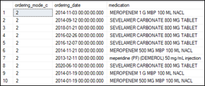
Figure 2.4: Intermediate Data from Basic Query Example.

2.3.3 Operators

Symbols specifying actions on expressions.

Various types of operators exist but operator types in the query example were arithmetic (*), comparison (=), logical (AND, BETWEEN, LIKE), and string (%).

2.3.4 Column and table aliases

User-defined alternative names for column or table names.

Column and table aliases must abide to SQL naming conventions (e.g., do not start with numbers, do not contain spaces, do not use reserved key words such as FROM or SELECT), otherwise the alias must be contained within brackets ([ ]). There are also some well described preferences within the SQL user community for naming conventions, including several popular style manuals, and even a dedicated ISO/IEC standard (ISO/IEC Joint Technical Committee 1/SC 32 2015), all of which will be covered in the section on

Table aliases can be referenced in subsequent query phases (e.g., in the SELECT phase when specifying column expressions like in Figure 2.1). For DBIs, column aliases are generally used for display or reporting purposes or referencing in complex expressions (e.g., queries with multiple SELECT statements that utilize previous query output for calculations).

Briefly, for Figure 2.1, ords.description was changed to medication and ords.hv_discrete_dose was changed to ordered_dose for clarity and preference — depending on the DBA, some RDMBS’s adopt less human-readable table and column names, which is often unacceptable for communicating results to others and can even be difficult for the individual SQL user to interpret their own code. Also note that the SELECT clause is followed by the ORDER BY clause; so, column aliases from the former query phase can be referenced in the latter.