Chapter 3 Building Isoscapes
3.1 Preparing the source data
To get an isoscape, you need data capturing how the isotope composition varies in space.
In this documentation, we will use data provided by the Global Network of Isotopes in Precipitation (GNIP), but you can use whatever source of data you prefer, or have access to.
In any case, do make sure to format your data the same way we do it.
Precisely, your dataset should be a data.frame (or a tibble) with the same columns as the ones shown below in section 3.1.2.
3.1.1 The GNIP database
You can download precipitation isotope data for hydrogen and oxygen from the Global Network of Isotopes in Precipitation (GNIP).
This step must be done outside IsoriX since there is no application programming interface for GNIP.
To get to know what the GNIP is, go there and explore related resources: https://www.iaea.org/services/networks/gnip
The GNIP data are free to download after the registration process is completed. The following link will bring you to the right place to create an account: https://websso.iaea.org/IM/UserRegistrationPage.aspx?returnpage=http://nucleus.iaea.org/wiser
Once your account has been activated, download the data you need from the WISER interface: https://nucleus.iaea.org/wiser/index (Tab Datasets)
Last time we checked, downloads were limited to 5,000 records per batch, which makes the compilation of huge databases fastidious.
GNIP promised to come up, in the future, with datasets directly prepared for IsoriX to save you the trouble.
We are eagerly waiting for this to happen!
3.1.2 A toy example: GNIPDataDE
Within IsoriX we have already included a small extract from GNIP corresponding to \(\delta^2H\) values for Germany.
The dataset has kindly been provided by Christine Stumpp and you can use it to try out the functions of the package without having to worry about getting data.
We won’t use this dataset here but it illustrates the structure of the data needed to fit an isoscape.
Here is what this dataset looks like:
3.1.3 A real example: GNIPDataEU
We are going to show you how to prepare a dataset for IsoriX starting from a raw extract from GNIP.
For this, we will use a file in which we have compiled the GNIP data for \(\delta^2H\) values for the whole world.
We are unfortunately unable to share these data with you, but you can download these data yourself as explained in section 3.1.1.
We first import the data into R:
This dataset contains 127637 rows and 24 columns. For example, the first row contains the following information:
| 1 | |
|---|---|
| Name.of.Site | NY ALESUND |
| Country | NO |
| WMO.Code | 100400 |
| Latitude | 78.91 |
| Longitude | 11.93 |
| Altitude | 7 |
| Type.Of.Site | Precipitation Collectors - not specified |
| Source.of.Information | [Partners: Sverdrup Station, Norsk Polarinstitutt], [Info: Major revision in 2013. All laboratory records from 1992-2009 replaced. Meteo data record replaced for 1991-2012 with official record from Norwegion Meteorological Office.] |
| Sample.Name | 199001 |
| Media.Type | Water - Precipitation - rain & snow (“mixed”) |
| Date | 1990-01-15 00:00:00 |
| Begin.Of.Period | 1990-01-01 00:00:00 |
| End.of.Period | 1990-01-31 00:00:00 |
| Comment | |
| O18 | -9.83 |
| O18.Laboratory | International Atomic Energy Agency, Vienna, AT |
| H2 | -72.8 |
| H2.Laboratory | International Atomic Energy Agency, Vienna, AT |
| H3 | 6.9 |
| H3.Error | 0.5 |
| H3.Laboratory | International Atomic Energy Agency, Vienna, AT |
| Precipitation | 27.6 |
| Air.Temperature | -6.4 |
| Vapour.Pressure | 2.6 |
We are now going to reshape these data step-by-step to make them ready for IsoriX.
We first reformat some temporal information:
rawGNIP$year.begin  <- as.numeric(format(as.Date(rawGNIP$Begin.Of.Period), "%Y"))
rawGNIP$year.end    <- as.numeric(format(as.Date(rawGNIP$End.of.Period), "%Y"))
rawGNIP$year.span   <- rawGNIP$year.begin - rawGNIP$year.end
rawGNIP$month.begin <- as.numeric(format(as.Date(rawGNIP$Begin.Of.Period), "%m"))
rawGNIP$month.end   <- as.numeric(format(as.Date(rawGNIP$End.of.Period), "%m"))
rawGNIP$day.span    <- as.Date(rawGNIP$Begin.Of.Period) - as.Date(rawGNIP$End.of.Period)
rawGNIP$Year        <- as.numeric(format(as.Date(rawGNIP$Date), "%Y"))
rawGNIP$Month       <- as.numeric(format(as.Date(rawGNIP$Date), "%m"))
Mind that, since we downloaded that file, WISER has renamed Begin.Of.Period to Begin.of.Period (small case for the “o” in of), so you may need to adjust that.
Do pay attention to other possible changes that may have also occurred in WISER.
Second, we identify the rows for which crucial information is missing. Because we are going to make an isoscape based on deuterium measurements, we only check for the availability of data for this isotope in particular. If you work on oxygen, you will have to adjust the script accordingly. We also check that the intervals during which precipitation water has been collected for each measurement corresponds roughly to one month:
rows_missing_or_unreliable_info <- is.na(rawGNIP$H2) |
                                   is.na(rawGNIP$day.span) |
                                   rawGNIP$day.span > -25 |
                                   rawGNIP$day.span < -35
Third, we only keep the rows and columns we are interested in:
columns_to_keep <- c("Name.of.Site", "Latitude", "Longitude", "Altitude",
                     "Year", "Month", "H2")
GNIPData <- rawGNIP[!rows_missing_or_unreliable_info, columns_to_keep]
Fourth, we turn the variable Name.of.Site into a factor:
Last, we rename the columns to conform to the general IsoriX format and we check that the data seems correct:
This is what the GNIPData looks like:
As you can see, the format is the same as the one for GNIPDataDE, which is precisely what we want.
3.2 Processing the source data
In order to build your isoscape with IsoriX, your dataset must be aggregated in such a way that each observation corresponds to the mean and variance of isotope values collected in one location, over a time period.
To aggregate the raw data, you can either choose to aggregate your dataset on your own (e.g. using the package dplyr), or to use our function prepsources().
This function allows you to apply some restriction on the data, such as selecting only particular months, years, or locations.
The function prepsources() also allows you to aggregate the data separately for different time periods (see section 6.3).
Each time period defines the temporal range of the data used to prepare a single set of isoscapes.
Most of the time people are only interested in a single time period (e.g. data over all years they have been collected), so we will not use this more advanced feature for this tutorial.
Here we use the function prepsources() to select from the dataset GNIPData the observations available across all years (i.e. a single time period) within an extent of latitude and longitude that covers roughly Europe.
This can be done as follows:
GNIPDataEUagg_test <- prepsources(data = GNIPData,
                                  long_min = -30, long_max = 60,
                                  lat_min = 30, lat_max = 70)
## Warning in prepsources(data = GNIPData, long_min = -30, long_max = 60, lat_min = 30, : The same combination of latitude, longitude and elevation correspond to different source_ID. Please consider fixing the data for the IDs:
## NIAMEY (ORSTOM), NIAMEY (IRD-IRI), SOROTI, BUGONDO, CAYENNE (FRENCH GUIANA), CAYENNE-SUZINI, BELEM, BELEM PIRACICABA, MANAUS, MANAUS PIRACICABA
## These IDs correspond to the following sets of lat long elev :
## -1.43 -48.48 24, -3.12 -60.02 72, 1.68 33.61 1038, 13.52 2.09 220, 4.83 -52.37 8As you can see, there are a few issues with the data. This is probably because the names used to refer to some weather stations have changed over time.
We therefore fix this by simply creating new values for source_ID in the original data and we then rerun prepsources():
GNIPData$source_ID <- factor(paste("site", GNIPData$lat, GNIPData$long, GNIPData$elev, sep = "_"))
GNIPDataEUagg <- prepsources(data = GNIPData,
                             long_min = -30, long_max = 60,
                             lat_min = 30, lat_max = 70)
No warning this time; that is better. Let us now explore the newly created dataset:
As you can see, we now have a single row of data per location.
The column mean_source_value gives the average across months and years.
The column var_source_value gives the variance between monthly measurements spanning across years.
3.3 Fitting the geostatistical models
Isoscapes are predictions stemming from statistical models.
In this section we will show you how to fit such models based on the dataset we prepared in section 3.2.
We refer to set of isoscapes because IsoriX does not create a single isoscape predicting the spatial distribution of isotopes (i.e. the main isoscape), but it also creates other isoscapes related to the main isoscape.
For example, it also creates an isoscape indicating how reliable the predictions are in any particular location.
If a single dataset is being used (as in section 3.2), then a single set of isoscapes needs to be built.
Instead, if several datasets have been prepared, then you will have to accordingly build multiple sets of isoscapes (see section 6.3 in this case).
To fit the geostatistical models required to build a single set of isoscapes, you need to use the function isofit().
The function isofit() has several parameters that can be adjusted to fit different models (see ?isofit).
Here we will consider two fixed effects (the elevation and the absolute latitude) on top of the default setting:
3.4 Saving the fitted models
Fitting models can take substantial computing time, depending on the amount of data you have and on the complexity of the models to be fit. Therefore, you may want to save the fitted models in order to be allowed to reuse them later (even after having opened a new R session), or in order to send them to your colleagues.
This can be done as follow:
The function saveRDS() will store your R object in a file.
To use saveRDS(), you must provide the object you want as a first argument of the function.
Then, file = defines the name of the file that will store the R object in your hard drive.
You can also include a path to this name so to store the file wherever you want.
This name can be different from the name of the object but here we stick to the same name for clarity.
The last argument compress = is optional; it allows for the creation of smaller files without loosing any content.
The only drawback of compressing is that the compression and the decompression can take some time.
Here the object is relatively quick to compress/decompress, so let us compress it and save a bit of space on the hard drive.
For loading a saved object (in a new session of R for example), just use the function readRDS() as follows:
Be careful, we do not recommend you to reuse saved objects after updating either IsoriX, or spaMM, or both.
After one of such updates, the best practice to make sure that every thing is working properly is to refit all your models.
By doing this you may also benefit from potentially new improvements we would have implemented.
There is another way to save and load objects in R, which is to use the function save() and load().
However, it is better to get used to the functions saveRDS() and readRDS() because only those can be used to store objects that contain spatial information (which we will do below).
3.5 Examining the fitted models
3.5.1 Plotting basic information about the models
You can display some information about the model fits by typing:
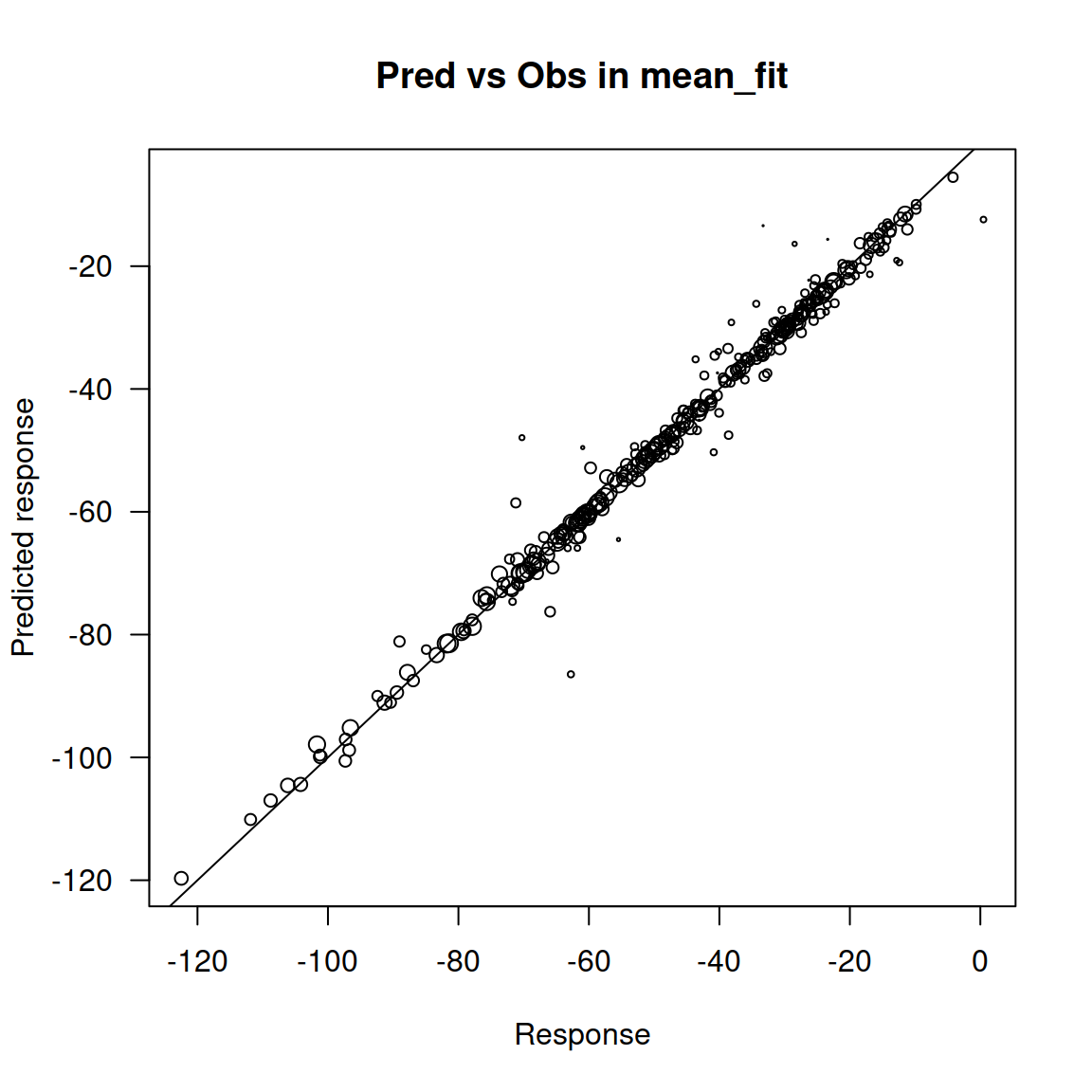
The first plot shows the relationship between the observed and predicted response for the fitted model called mean_fit, which corresponds to the fit of the mean isotopic values.
The second plot shows the same thing for the model called disp_fit, which corresponds to the fit of the residual dispersion variance in the isotope values.
Here you can see, in these first two plots the points are distributed practically along the 1:1 diagonal.
A different slope would suggest a high residual variance of the data.
We do not expect the points to fall exactly on the 1:1 line because the model fit does not attempt to predict perfectly the observations used during the fit.
Instead, the model fit produces a smooth surface that aims at reaching a maximum predictive power for locations not considered during the fit.
The third and fourth plots show the variation in spatial autocorrelation with the distance between locations captured by mean_fit and disp_fit, respectively.
These plots thus give you an idea of the strength of the spatial autocorrelation captured by the models.
Here the results suggest that the autocorrelation is very strong.
Not considering this autocorrelation would thus lead here to a poor approximation of the isoscape and resulting assignments.
3.5.2 Examining the summary tables
To explore the fitted models you can start by simply typing their name and the information of each fit will be displayed:
##
## ### spaMM summary of the fit of the mean model ###
##
## formula: mean_source_value ~ 1 + elev + lat_abs + (1 | source_ID) + Matern(1 |
##     long + lat)
## REML: Estimation of corrPars and lambda by REML.
##       Estimation of fixed effects by ML.
## Estimation of lambda by 'outer' REML, maximizing restricted logL.
## family: gaussian( link = identity )
##  ------------ Fixed effects (beta) ------------
##             Estimate  Cond. SE t-value
## (Intercept)  65.0326 3.412e+01   1.906
## elev         -0.0106 8.132e-04 -13.031
## lat_abs      -2.3374 4.467e-01  -5.233
##  --------------- Random effects ---------------
## Family: gaussian( link = identity )
## Distance(s): Earth
##                    --- Correlation parameters:
##         2.nu        2.rho
## 3.197883e-01 3.024525e-05
##            --- Variance parameters ('lambda'):
## lambda = var(u) for u ~ Gaussian;
##    source_ID  :  1e-05
##    long + lat  :  987.6
## # of obs: 327; # of groups: source_ID, 327; long + lat, 326
##  -------------- Residual variance  ------------
## Prior weights: 19 17 5 1 17 ...
## phi was fixed [through  "phi" ~ 0 + offset(pred_disp) ] to 341.334 292.434 384.211 406.772 262.825 ...
##  ------------- Likelihood values  -------------
##                         logLik
## logL       (p_v(h)): -1103.073
## Re.logL  (p_b,v(h)): -1104.910
## NULL
##
##
## ### spaMM summary of the fit of the residual dispersion model ###
##
## formula: var_source_value ~ 1 + (1 | source_ID) + Matern(1 | long + lat)
## Estimation of corrPars and lambda by REML (P_bv approximation of restricted logL).
## Estimation of fixed effects by ML (P_v approximation of logL).
## Estimation of lambda by 'outer' REML, maximizing restricted logL.
## family: Gamma( link = log )
##  ------------ Fixed effects (beta) ------------
##             Estimate Cond. SE t-value
## (Intercept)    5.883    1.942    3.03
##  --------------- Random effects ---------------
## Family: gaussian( link = identity )
## Distance(s): Earth
##                    --- Correlation parameters:
##         2.nu        2.rho
## 3.122037e-01 1.477985e-05
##            --- Variance parameters ('lambda'):
## lambda = var(u) for u ~ Gaussian;
##    source_ID  :  3.635e-05
##    long + lat  :  4.404
## # of obs: 322; # of groups: source_ID, 322; long + lat, 321
##  --- Residual variation ( var = phi * mu^2 )  --
## Prior weights: 18 16 4 16 77 ...
## phi was fixed to 2
##  ------------- Likelihood values  -------------
##                        logLik
## logL      (P_v(h)): -2066.554
## Re.logL (P_b,v(h)): -2064.972
## 2.rho are at their lower optimization bound.
## NULL
##
## [models fitted with spaMM version 4.5.0]
##
## NULL
The object EuropeFit created in section 3.3 is a list containing the two fits aforementioned: mean_fit and disp_fit.
This is why you see information about those two corresponding fits.
These summary tables are created behind the scenes by spaMM, so, learning a little about spaMM and mixed models is useful to derive meanings from these outputs.
(We are also planning to write an extensive description of model outputs to guide you.)
3.5.3 Doing more stuff with the fitted models
Each of the fitted models is an object of class HLfit which has been created by spaMM.
You can thus directly manipulate those fits using spaMM for advanced usage.
For example, if you want to compare different models using the information criterion, you can call the AIC() function implemented by spaMM by simply typing:
##        marginal AIC:     conditional AIC:      dispersion AIC:
##            2220.1461            1840.6432            2217.8208
##        effective df:
##             106.5232
Note that we re-exported some spaMM functions for you to use without the need to load the package spaMM (e.g. AIC.HLfit() which is implicitly here), but you will have to call library(spaMM) to access all spaMM functions.
3.6 Building the isoscapes
3.6.1 Prepare the structural raster
To build the isoscape using the geostatistical models fitted above, you need to provide the function isoscape() with a structural raster.
Such raster defines the locations at which we want to predict the isotopic values.
It must also contain the values for the predictors used in the geostatistical models at such locations.
We will thus start by preparing such structural raster.
Here, as a basis for the structural raster, we will download a high resolution elevation raster from the internet using our function getelev:
You may not need to pass any argument to getelev(), but here we chose to define ourselves where to store the elevation raster and how to call such file using file = "input/elevation_EU_z5.tif".
We did not alter the default resolution, which is high enough for our example, but doing so would be easy: one simply needs to define a value lower or larger than 5 for the zoom parameter z (see ?getelev() for details and here for information on what the value for the zoom parameter z really implies).
We then import the high resolution elevation raster and transform it into an R object of class SpatRaster using the package terra:
## we import the high resolution raster
ElevWorld <- rast("input/elevation_world_z5.tif")

## we check that the import worked
ElevWorld
## class : SpatRaster
## dimensions : 9899, 20950, 1 (nrow, ncol, nlyr)
## resolution : 0.0171833, 0.01718412 (x, y)
## extent : -180, 179.9902, -85.05449, 85.05113 (xmin, xmax, ymin, ymax)
## coord. ref. : lon/lat WGS 84 (EPSG:4326)
## source : elevation_world_z5.tif
## name : elevation_world_z5
## min value : -10697
## max value : 7963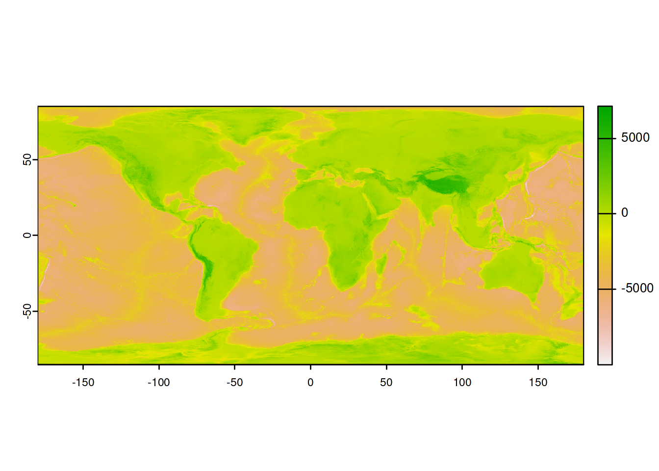
Then, you may need to crop and resize this raster to the appropriate size before creating the isoscapes.
Cropping is used to define a rectangular area over which we will predict the isotope values. If the area you define to build your isoscapes is too small, you may miss crucial information. For example, a set of isoscapes that covers an area that is too small may lead you to miss the real origin of your migratory organisms during the assignment step. Similarly, if the area to be used for building the isoscapes is too large, you may extrapolate and the model will thus create unreliable predictions.
Resizing the raster is used to reduce its resolution by aggregating neighboring cells.
If the selected resolution is too large, computations may take too much time or memory to work.
If the selected resolution is too coarse, you may smooth too much the predictors over the landscape (e.g. the peaks and valleys of a mountain chain will be reduced to a plateau), which will lead to unrealistic isoscapes that are too smooth.
To crop and resize the structural raster, you can use our function prepraster().
Geeky note: In principle you could directly crop and resize the raster to the dimensions you want before downloading it (getelev() does allows for you to do that).
However, in practice, we recommend you to download a raster that is a little larger than what you need (getelev() downloads the full world by default, which should always be sufficient) and with a resolution overshooting a little what you may need.
The benefit of relying on prepraster() rather than getelev() to crop and downsize the structural raster is that you can study the impact of your decisions by simply rerunning prepraster() again – with different settings – without having to download again a large amount of data from the net.
Here, the structural raster downloaded with getelev() covers the entire planet, so we will crop it to the limits of Europe, which we also used to select our source data (see section 3.2).
To crop the elevation raster to a particular size, you can either provide a set of coordinates to prepraster()by means of the argument manual_crop.
Alternatively, you can simply provide a fitted model to the function prepraster() by means of the argument isofit.
In this latter case, the function will automatically determine the coordinates required for the cropping, from the coordinates of the weather stations used during the fitting procedure.
We choose here to use this simpler way of defining the cropping area:
You may see that we also reduced the resolution of the elevation raster by choosing an aggregation factor of 4.
We recommend to first use a large aggregation factor (e.g. 10) to draft your workflow and quickly notice errors in your code.
Once things are working as they should, we recommend you to then use the lowest aggregation factor that your hardware and patience can handle (i.e. 0 if possible).
As mentioned above, if you need isoscapes with an even greater resolution, use getelev() with a value of the parameter z that is higher than 5 (an increment of 1 – i.e. z = 6 already makes a big difference as shown here).
Here we set the aggregation_factor to 4 to produce plots nice enough for this tutorial, without being too heavy for us to recompile this bookdown quickly; but, for real applications, you should use a higher resolution.
You can easily check what your structural raster looks like by plotting it.
Compared to the map plotting above for ElevWorld, we will now draw a slightly more advanced map using the functions of the packages lattice and rasterVis which we made available in IsoriX:
levelplot(ElevEurope,
          margin = FALSE,
          col.regions = viridisLite::turbo, ## the colour palette
          main = "Structural raster") +
layer(lpolygon(CountryBorders, border = "white")) +
layer(lpolygon(OceanMask, border = "white", col = "lightgrey"))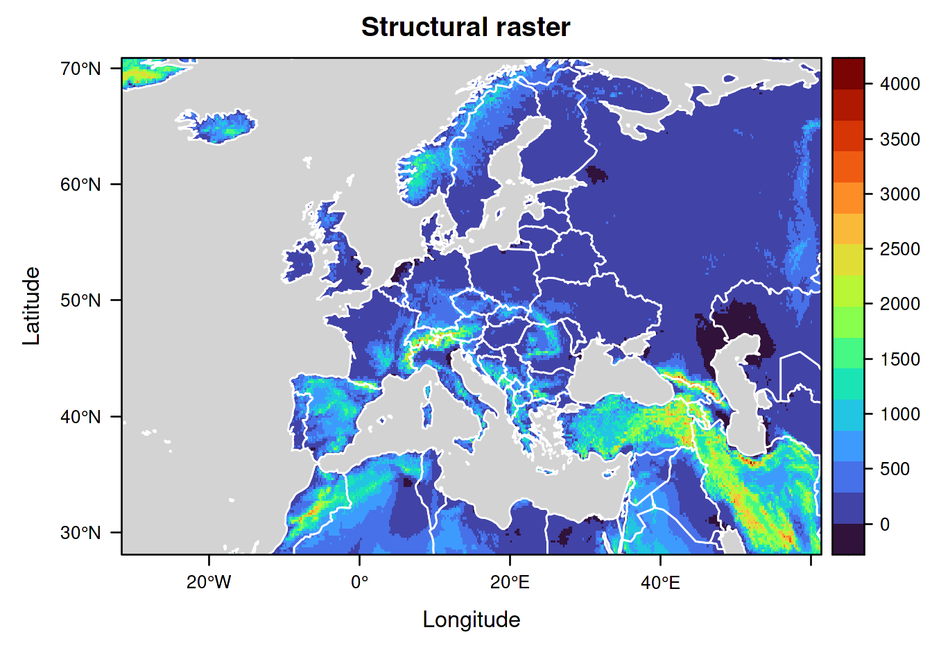
Note that, in this raster, the highest elevation does not correspond to the actual highest elevation known in the depicted area (the maximal value in the raster is 4113m, but Mount Elbrus is 5642m high). This is not a bug but an expected result of aggregation. Indeed, each cell of the raster only contains a single value which corresponds to a summary statistic (the mean) applied to all locations aggregated together in the cell.
Geeky note: You may change what summary statistic is applied when using prepraster() using the argument aggregation_fn, but you have no control over the aggregation happening within getelev() since it uses ultimately a package that does not allow for controlling the summary statistics.
Whatever you do, think carefully on the consequences of your choice upon how you are planning to use the isoscapes (e.g. for assigning species living only at the top of the mountains, using aggregation_fn = max may make more sense than the default).
3.6.2 Predicting the isoscapes
We will now build the isoscapes using the function isoscape().
The function simply takes the structural raster and the fitted model as arguments:
The function isoscape() creates 8 different rasters that correspond to different aspects of the isoscape (see ?isoscape() for details).
We can check which rasters have been created by typing:
## class       : SpatRaster
## dimensions  : 623, 1352, 8  (nrow, ncol, nlyr)
## resolution  : 0.06873321, 0.06873649  (x, y)
## extent      : -31.55346, 61.37383, 28.08577, 70.9086  (xmin, xmax, ymin, ymax)
## coord. ref. : +proj=longlat +datum=WGS84 +no_defs
## source(s)   : memory
## names       :        mean, mean_predVar, mean_~idVar, mean_respVar,       disp, disp_predVar, ...
## min values  : -124.359990,     2.875243,    66.75802,     70.27486,   66.75802,   0.01258517, ...
## max values  :    5.775813,   223.085668,  1557.88997,   1576.86819, 1557.88997,   0.60288326, ...
3.7 Plotting the isoscapes
One particular strength of IsoriX is the ability to produce nice looking and highly customisable plots of the isoscapes and assignment maps.
All plotting functions in IsoriX present default settings so that a simple call to plot() on your object is sufficient to generate a nice looking plot.
For example, here you can obtain the main isoscape by typing:
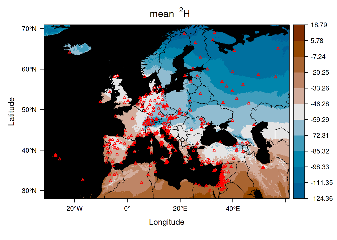
This shows the prediction of the average isotope value in space (i.e. the point prediction).
For more information about how to improve your plots, check the section 6.1.
3.7.1 Other isoscapes
You can also plot any of the other isoscapes by specifying the name of the raster using the argument which.
As examples, we are now going to plot the residual variation in isotope values predicted at each location, and the prediction variance:
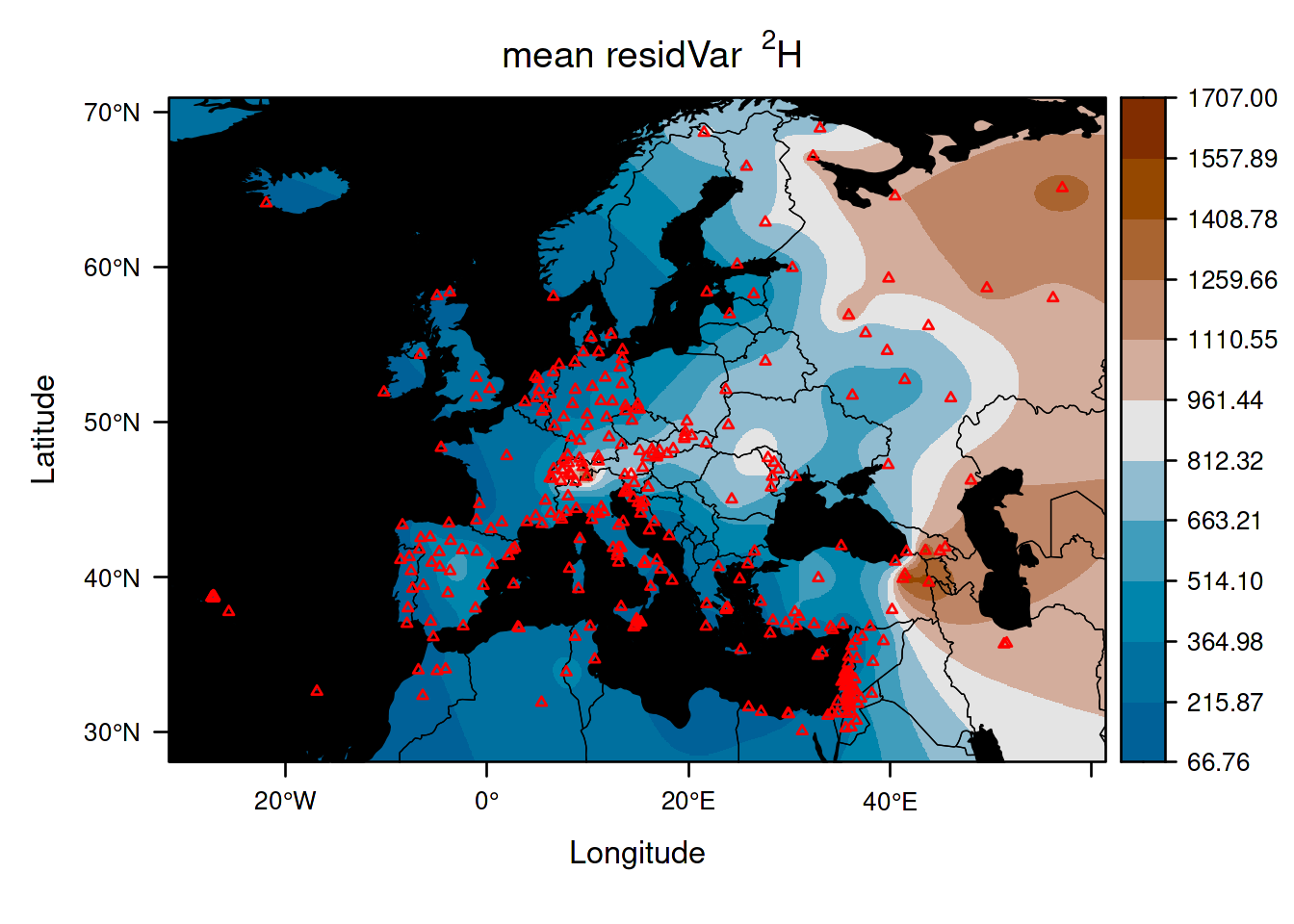
This first isoscape quantifies the temporal variation at each location.
Here the variation represents the between month variance spanning across years, but it will not always be so as it depends on how you aggregated the data (see section 3.2).
Interestingly, you can see that the variance is large and spatially structured.
Believe it or not, but most methods of assignment alternative to IsoriX consider such variance to be equal to zero!
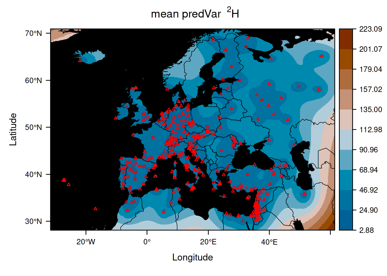
This second isoscape quantifies the uncertainty in your point predictions. As you can see, the uncertainty increases when you go far from the source location. This isoscape can help to update the design of the data collection. It is also used internally when performing assignment. Indeed, if you are very uncertain of what the average isotope value is in a location, then you cannot rule out that any organism may have come from that location. It is unfortunate but an inescapable reality.