Chapter 5 Inferring geographic origins
We will now show how to perform the geographic assignment as such. For this, you need the isoscapes built as shown in chapter 3 and the isotope data of the assignment samples. If the type of samples you want to assign differ from the type of samples you used to create the isoscapes, then you will also need a calibration fit obtained as shown in chapter 4.
5.1 Preparing the data
You need at least two pieces of information from the samples that you want to assign: a label and an isotope value.
You should provide such information as a data.frame with the column names sample_ID and sample_value.
You may also add the latitude and longitude of the sampling locations for the assignment samples, if you want that such locations appear on your assignment maps.
However, such locations are not considered for the statistical assignment.
Here we are going to assign the following bats:
| sample_ID | lat | long | sample_value |
|---|---|---|---|
| Nnoc_1 | 51.72323 | 13.67630 | -43.40550 |
| Nnoc_2 | 51.72323 | 13.67630 | -49.59752 |
| Nnoc_3 | 51.72323 | 13.67630 | -45.19298 |
| Nnoc_4 | 51.69520 | 14.64945 | -41.95605 |
| Nnoc_5 | 51.70366 | 14.63915 | -58.19690 |
| Nnoc_7 | 51.69520 | 14.64945 | -42.56502 |
| Nnoc_8 | 51.70536 | 14.63289 | -46.26581 |
| Nnoc_9 | 51.70536 | 14.63289 | -48.47353 |
| Nnoc_10 | 51.89348 | 13.76488 | -42.53986 |
| Nnoc_11 | 51.84883 | 13.64525 | -43.79554 |
| Nnoc_12 | 51.60535 | 11.92700 | -45.72407 |
| Nnoc_13 | 51.96695 | 12.08462 | -57.72157 |
| Nnoc_15 | 51.96695 | 12.08462 | -72.43155 |
| Nnoc_16 | 51.45457 | 11.50689 | -53.39763 |
This dataset is available in IsoriX.
It contains hydrogen delta values of fur keratin from common noctule bats (Nyctalus noctula) killed at wind turbines in northern Germany.
The question we want to answer is whether those bats are local bats or migratory bats killed during their migration.
5.2 Running the geographic assignments
Running the assignment is fairly straightforward: you must use the function isofind() and provide it with the data frame containing the data to assign, the isoscape object (i.e. the object produced by the function isoscape(); see chapter 3), and (if needed) the calibration object (i.e. the object produced by the function calibfit(); see chapter 4):
The output of the function, here stored under the name AssignedBats, is a list of class ISOFIND containing 3 elements: the element sample storing all rasters related to the assignment of each single sample, group storing the rasters related to the group assignment, and sp_points storing the spatial points of the source locations as well as the ones for the calibration samples and the assignment samples (if available).
As for the output of the function isoscape(), we choose to store all this information in a single R object to make the plotting of the assignment maps easy peasy.
5.3 How does the assignment work?
Here we explain how the assignment procedure works without going into geeky details. It is important that you understand how it works because it has bearing on how you must interpret the assignment results.
First, isofind() runs the assignment test for each sample at each candidate location or cell from our structural raster.
Precisely, for each candidate location the function tests whether the isoscape value at the unknown location of origin of a given sample is consistent with the predicted isoscape value at the candidate location.
To do this, we use the difference between these two isoscape values as a test statistic.
The isoscape value at the unknown location of origin is either the isoscape value of the assignment sample if no calibration is being supplied (when the source samples and assignment samples are of the same type), or isofind() computes it by inverting the calibration relationship established by the calibration fit (when a calibration is required; see chapter 4).
The predicted isoscape value of the candidate location is directly the point prediction of the isotope value at each prediction location, which is an information given by the main isoscape (see chapter 3).
The test statistics over all locations can be retrieved for each sample from the object produced by isofind().
For example, the raster stored under the name AssignedBats$sample$stat$Nnoc_1 contains such information for the first bat:
## class       : SpatRaster
## dimensions  : 623, 1352, 1  (nrow, ncol, nlyr)
## resolution  : 0.06873321, 0.06873649  (x, y)
## extent      : -31.55346, 61.37383, 28.08577, 70.9086  (xmin, xmax, ymin, ymax)
## coord. ref. : +proj=longlat +datum=WGS84 +no_defs
## source(s)   : memory
## name        :    Nnoc_1
## min value   : -60.16976
## max value   :  63.46147
We now detail the variance associated to the test statistic.
Under the null hypothesis, we just saw that the isotope value at location of origin equals the isotope value at the candidate location. The variance of the test statistic is thus the variance of the difference between these two isoscape values.
The variance of the test statistic is also stored as a raster (e.g. AssignedBats$sample$stat_var$Nnoc_1).
In the appendix of our book chapter (Courtiol et al. 2019), we show that such variance of the assignment test depends on up to four terms (some may be omitted depending on the calibration method considered):
The prediction variance of the mean fit, which is not constant over the entire spatial range (see Appendix). Therefore, a small difference in isoscape values at a location where the prediction variance is very small may argue against an assignment at the corresponding location, while a large difference where the prediction variance is very large may not.
The residual variation among samples at the unknown location of origin. In the workflow illustrated here, we estimate such variance from the residual variance of the calibration fit, which we assume constant. Other approaches are possible in
IsoriX. In particular, if assignment samples are of the same kind as the source sample (and thus when no calibration model exists), such variance is instead given by the residual dispersion variance of the isoscape.The prediction variance of the calibration fit (which decreases with the size of the calibration dataset) given the predicted isoscape value at the candidate location.
A covariance term between the prediction error of the calibration fit given the predicted isotope value at the candidate location, and the prediction error of the isoscape at this location. We can compute this last term, which relates the uncertainty of the isoscape to the one of the calibration in
IsoriX, because the calibration and the geographic assignment are both computed within the same software package.
For each candidate location of origin, the p-value of the assignment test is the probability that an assignment sample truly originating from the candidate location has a larger absolute value than the observed test statistic.
Even if a location presents a perfect match (p-value close to one), it does not mean that the location is the true place of origin.
It only means that the candidate location has an isotopic composition similar to the location of true origin, irrespective of where this location may be.
This limitation is of course not specific to IsoriX.
The p-value of the assignment test is also stored in a raster within the object produced by isofind() (e.g. AssignedBats$sample$pv$Nnoc_1) and you can use such raster to directly extract the result of the test of an assignment hypothesis.
For example, to test whether the first bat to assign (Nnoc_1) originates from its sample location we can simply type:
The outcome of this call gives a non-significant p-value, so we cannot rule out a local origin for the first bat.
Repeating this for all assignment samples shows that we only reject a local origin for the bat Nnoc_15:
Pvalues <- sapply(1:nrow(AssignDataBat),
                  function(i) extract(AssignedBats$sample$pv[[i]],
                                       cbind(AssignDataBat$long[i],
                                             AssignDataBat$lat[i])))
AssignDataBat$sample_ID[Pvalues <= 0.05]
## [1] Nnoc_15
## 14 Levels: Nnoc_1 Nnoc_10 Nnoc_11 Nnoc_12 Nnoc_13 Nnoc_15 Nnoc_16 ... Nnoc_9The assignment function isofind() always performs two types of geographic assignments: an individual assignment and a group assignment.
The individual assignment which we have just explored is useful to infer the origin of a single sample or to infer independently the origin of several samples.
In contrast, the group assignment infers a single origin for all the samples in the data frame.
The underlying assumption of a group assignment is that all the individuals come from the same location of origin.
Note: if you wish to assign different groups of samples separately, you simply have to prepare several data frames and run the assignment function on each of the groups separately.
Once the function isofind() has assigned all samples individually, it thus performs the group assignment.
The p-value of the geographic assignment test for the entire group (here stored as the raster AssignedBats$group$pv) is computed by combining, at each location, the p-values of the geographic assignment for all assignment samples using Fisher’s combination of probabilities method (Fisher 1925).
The null hypothesis of this group assignment is that all assignment samples originate from a location with identical distribution of source isotope values as the one being tested. Therefore, the test considers that all assignment samples must come from the same location of origin (or at least from a set of locations presenting the same isotopic composition), and if this assumption is not fulfilled, the test may exclude all candidate locations. This is why you should always start by exploring individual assignments even if you are ultimately interested in a group assignment.
5.4 Plotting the geographic assignments
You can plot the geographic assignments by simply calling the generic function plot().
The generic function will invoke a plotting method very similar to the one described for isoscapes (section 6.1.2).
Most arguments between the two plotting methods are the same.
They are detailed in the help file ?plots.
One main difference, however, is that the argument which used to indicate which raster to plot (mean, mean_predVar, …) is now replaced by an argument who.
If you set who to "group", the function will show a single map representing the geographic assignment for the group.
If instead you want to obtain a single assignment map per sample, you can provide a vector of the samples to be plotted (as indices or using their ID) to who .
Here is an example for plotting the first 2 bats:
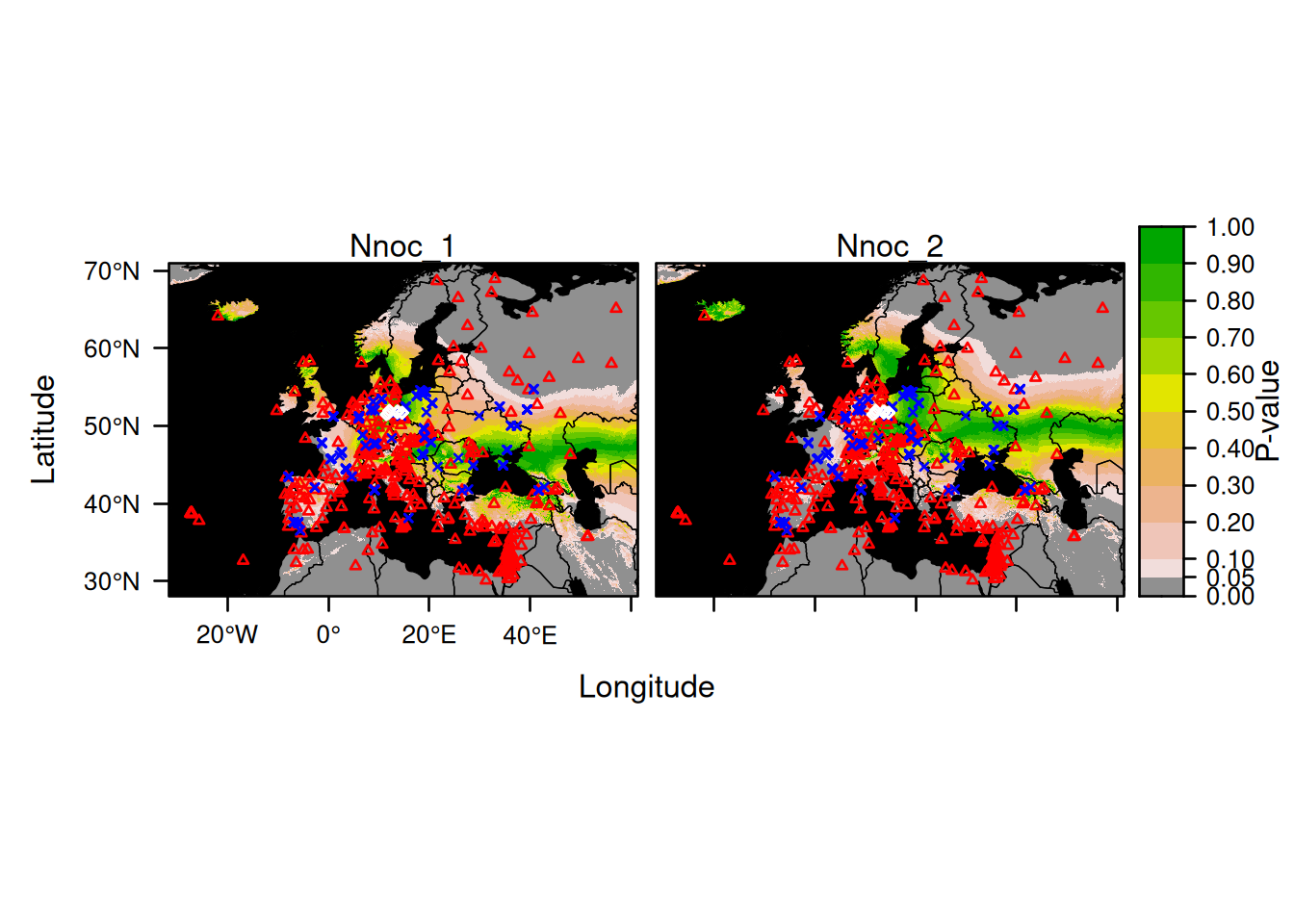
Here is an example for plotting explicitly all 14 bats:
plot(AssignedBats,
     who = 1:14,
     sources = list(draw = FALSE),
     calibs = list(draw = FALSE),
     assigns = list(draw = FALSE)
     )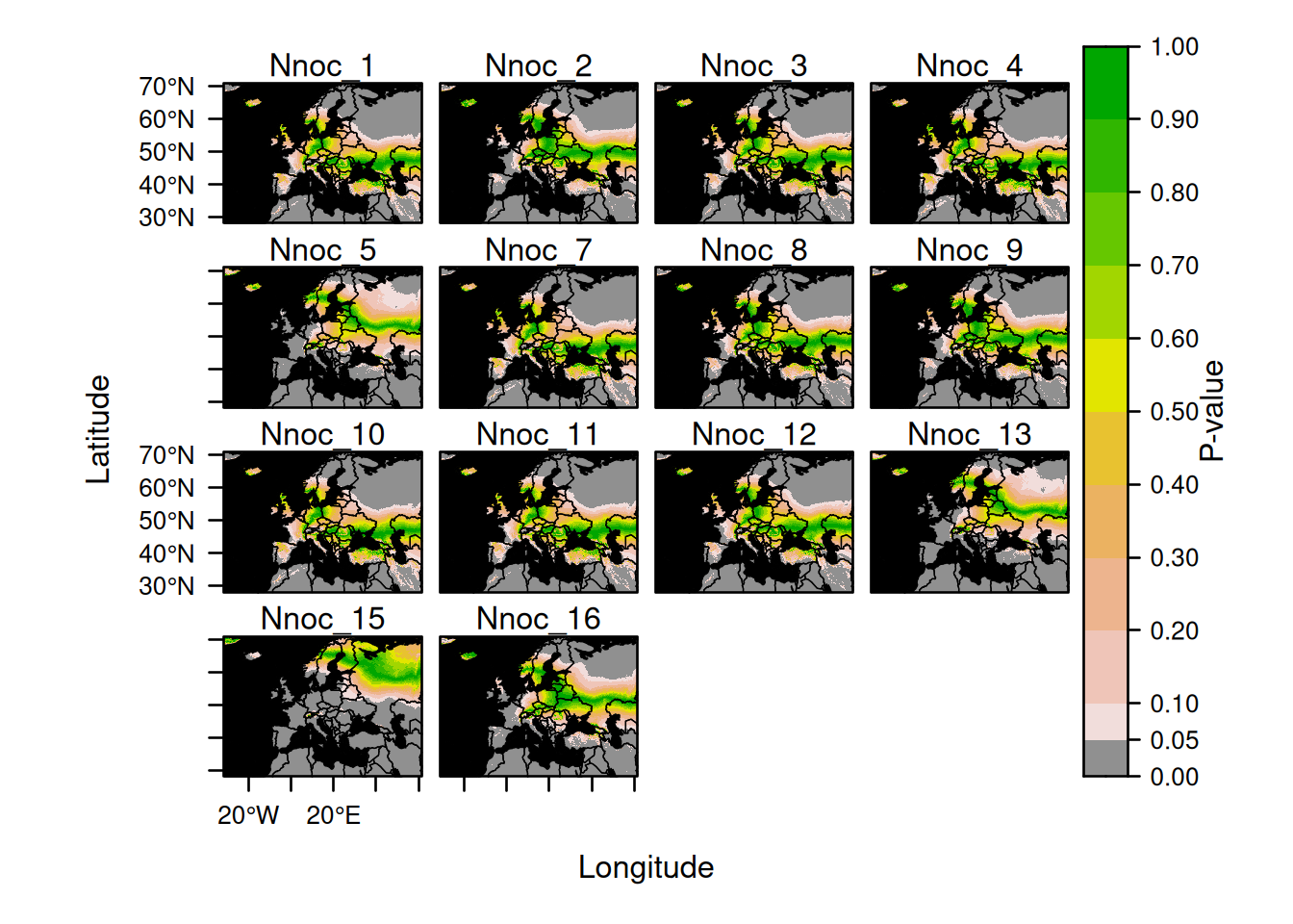
Note that we used the arguments sources, calibs and assigns to prevent the automatic display of points which would saturate the tiny maps.
Here is an example showing how to plot a specific sample using its name:
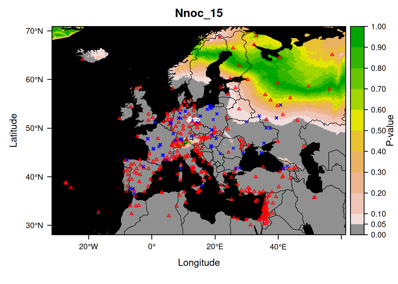
We did not choose the bat randomly.
As you can see, this probability map confirms what we found above: the sampling location (eastern Germany) being rejected as a source of origin for the bat Nnoc_15.
We will now make a group assignment:
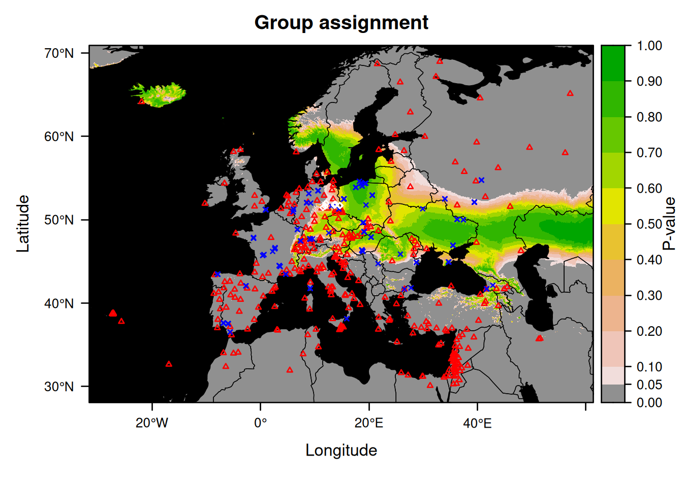
This map does not make much sense if the bats come from different locations.
So instead, we will now rerun the assignment and plot the result after taking out the individual that is likely to originate from outside Germany (Nnoc_15).
This can be done by typing:
AssignDataBat2 <- subset(AssignDataBatRev, sample_ID != "Nnoc_15")
AssignedBats2 <- isofind(data = AssignDataBat2,
                         isoscape = EuropeIsoscape,
                         calibfit = CalibBats)
## [1] "computing the test statistic and its variance..."
## [1] "running the assignment test..."
## [1] "combining assignments across samples..."
## [1] "assignments for all 13 organisms have been computed in 6s."
## [1] "converting log p-values into p-values..."
## [1] "applying the mask..."
## [1] "done!"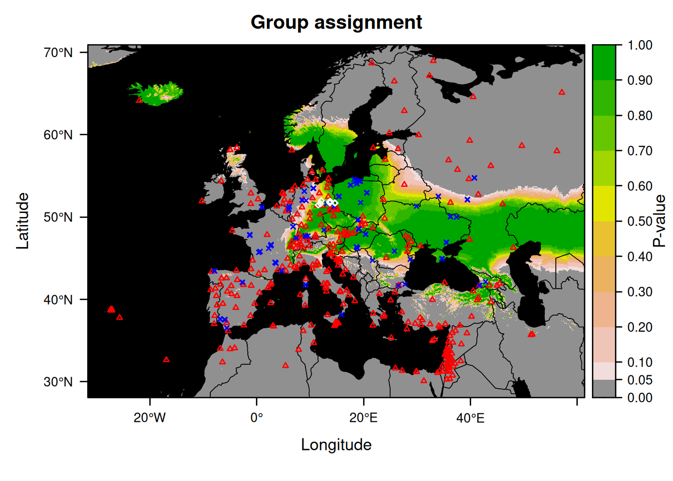
5.4.1 More information on the assignment plots
The plotting method uses the information from the assignment test to define confidence regions.
By default, a region corresponding to the most unlikely 5% is being displayed in grey, which means that the non-grey areas should contain the true location of origin with a 95% probability.
You can alter this setting using the argument level.
Another default setting considered by IsoriX, is to apply a mask to hide the outcome of the geographic assignment over the large water bodies.
You can change that as well using the argument mask.
Related to these arguments, you can also define another mask using the argument mask2.
You may want to use it, for example, to hide areas outside the IUCN distribution map for your species.
If more than two masks are necessary, just combine several masks into one and provide that one to the argument mask2.
For plotting, if these extra masks need to be visually distinct, you can use the function layer() and lpolyong() similarly to what we did towards the end of section 3.6.1.