Chapter 5 Inventory Models with Stochastic Demand
Following the two main criteria described in Chapters 2 and 3, there are different inventory models that can be adjusted form standard to modified situations.
As mentioned in the Chapter 2, there are two main types of demand: Deterministic and Stochastic. For cases with stochastic demand, the demand is unknown or uncertainty, and it is modeled with a probability distribution. This probability distribution can be a normal, poisson, uniform, and more. According to Silver, Pyke, and Thomas (2017), the three key issues to be resolved by a control system under stochastic demand are:
- How often the inventory status should be determined.
- When a replenishment order should be placed.
- How large the replenishment order should be.
Under stochastic demand, the demand can change unexpectedly and it is more important to get systems to track the inventory level, compared with the deterministic demand, where the inventory level is expected. For this reason, the first key (Silver, Pyke, and Thomas (2017)) is more complicated with stochastic demand, where resources like labor and computer time are needed. The less the inventory level is checked, the most protection against unexpected variations on the demand (Silver, Pyke, and Thomas (2017)).
Due to the uncertainty of demand, a safety stock is usually used to replenish the expected demand and reduce shortages. Regarding the shortages, there are two principal structures:
- Backorders: it is the demand that cannot be served because of not enough stock, but is served in the next cycle when stock is available again.
- Lost sales: it is the demand that cannot be served because of not enough stock, and is not served in next cycles, it means, it becomes lost sales.
In classic models, generally it is assumed that the demand not served is backorder, however, studies have shown that demand not satisfied is more common to be a lost sale (Prado-Prado and García-Arca (2012)).
Inventory control models with stochastic demand are divided into two main categories, as shown in Chapter 3: continuous and periodical review (Prado-Prado and García-Arca (2012)). A continuous revision system is when the inventory level can be known all the time, instead of the periodical, where the inventory level is not reviewed constantly, only every \(t\) amount of time.
In stochastic demand, two service levels are considered (Axsäter (2015)):
- Service Level Type I (\(\alpha\)): this service level refers to the probability of not having shortages or the portion of cycles without shortages.
- Service Level Type II (\(\beta\)): this service level refers to the portion of the demand satisfied with the units in stock.
5.1 Stochastic Demand in Continuous Revision Systems
As shown in Chapter 3.1, this revision system tracks all the time the inventory level. It means that it is known when an unit arrives or leaves the storage.
5.1.1 QR Model
The QR model is an important model in the literature (Prado-Prado and García-Arca (2012); Silver, Pyke, and Thomas (2017)), this model gets as a result the quantity to order \(Q\) every time the inventory level reaches the reorder point \(R\). It is important to know that the inventory level measures the ability to satisfy the future demand (Prado-Prado and García-Arca (2012)). The QR model is also called two-bin system (Silver, Pyke, and Thomas (2017)): in one bin is the reorder point \(R\) amount of units and in the other bin is the rest of the inventory level, once the second one is finished, and order is placed and the first bin is used to fulfill the demand while the order placed arrives. When the order arrives, the first bin is filled until reached the reorder point \(R\) amount and the rest goes to the second bin.
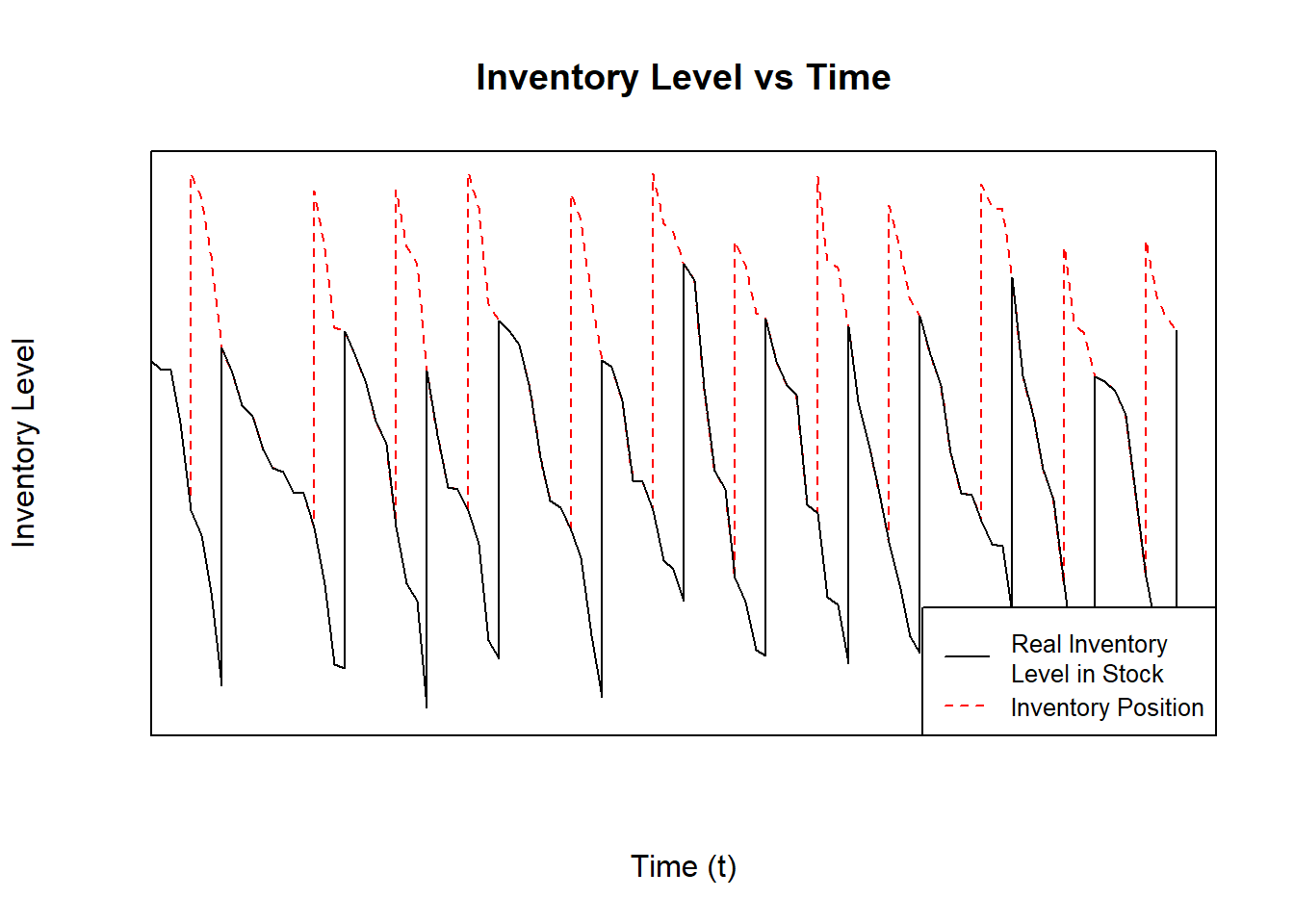
Figure 5.1: Inventory Level in a QR Model With Stochastic Demand
In Figure 5.1 are shown two plots, the black and dashed red lines. The black line shows the real inventory level available in stock and the dashed red line shows the position of the inventory including orders that have not arrived yet. In this figure, the stochastic demand can be observed, the inventory level does not decrease in a constant rate.
The main purpose of the QR model is to find an optimal reorder point \(R\) and a optimal order quantity \(Q\) each time the inventory level (black line in Figure 5.1), To do so, it is important to consider the next important keys:
- The time an order takes to arrive since it is placed is called Lead Time \(\tau\).
- The demand is stochastic and stationary. It can be modeled by a probability distribution and does not have trend or seasons.
- The inventory level can be reviewed all the time (continuous review system).
The importance of \(R\) in this model is to ensure that there is enough inventory to cover the demand during the Lead Time \(\tau\), and the order quantity \(Q\) makes sure that the model gives the economical solution, because, if the quantity \(Q\) is small, orders should be placed more often, and if the quantity \(Q\) is large, the holding costs would be high. In QR Model, there must be a balance between \(Q\) and \(R\).
The optimal policy for the QR model can be found using one of the next two equations (Axsäter (2015)):
With Backorders System: \[\begin{equation} F(R) = \alpha = 1 - \frac{Qh}{p\lambda} \tag{5.1} \end{equation}\] Where \(Q\) is the optimal order quantity, \(h\) is the holding cost per item per time, \(p\) is the cost of a shortage in the stock or the money that won’t be received due to a shortage, and \(\lambda\) is the mean of the demand (independent of the probability distribution).
With Lost Sales System: \[\begin{equation} F(R) = \alpha = 1 - \frac{Qh}{Qh+p\lambda} \tag{5.2} \end{equation}\] Where \(Q\) is the optimal order quantity, \(h\) is the holding cost per item per time, \(p\) is the cost of a shortage in the stock or the money that won’t be received due to a shortage, and \(\lambda\) is the mean of the demand.
To begin with the model, the amount of \(R\) should be enough to cover the demand during Lead Time \(\tau\). The next steps should be followed:
It is necessary to calculate a first approximate order quantity \(Q\) based on the Equation (4.4): \[Q_1 = EOQ = \sqrt{\frac{2K\lambda}{h}}\] Where \(K\) is the cost for every order placed.
The next step is to calculate the service level type I \(\alpha\) or, in this case, \(F(R)\) based on the Equations (5.1) or (5.2). Then, the reorder point \(R\) can be calculated depending on the probability distribution and considering that \(F(R)\) is the accumulated probability of \(R\).
After finding the reorder point \(R\), the expected value of shortages \(n(R)\) can be calculated with the next equation: \[\begin{equation} n(R) = \int_R^\infty{(x_\tau - R)f(x_\tau)dx_\tau} \tag{5.3} \end{equation}\]
Once steps 1 to 3 has been followed, the order quantity now can be calculated including the shortages cost: \[\begin{equation} Q = \sqrt{\frac{2\lambda(K+pn(R))}{h}} \tag{5.4} \end{equation}\]
Repeat the steps 2 to 4 until \(Q\) and \(R\) converge and do not change significantly between repetitions.
The average total cost expected is based on the Equation (4.1) adding the cost of shortages:
\[G(Q) = \frac{K}{T} + \frac{cQ}{T} + h\overline{I} + \frac{pn(R)}{T}\]
In this case, due to the uncertainty of the demand, it is possible to suppose that \(\lambda = \frac{Q}{T}\), and the average inventory \(\overline{I}\) will be \(\overline{I} = \frac{Q}{2} + SS\), where \(SS\) is the safety stock calculated depending on the sales system:
- With Backorders system, \(SS = R - \lambda_\tau\), where \(\lambda_\tau\) is the expected demand in the Lead Time (\(\tau\)) period.
- With Lost Sales system, \(SS = R - \lambda_\tau + n(R)\), where \(\lambda_\tau\) is the expected demand in the Lead Time (\(\tau\)) period.
In the Backorders system, the safety stock \(SS\) can be negative, which means there are some missing units that should be satisfied when the next order arrive. However, in the Lost Sales system, the safety stock \(SS\) must be \(0\) or positive, because once the demand can not be cover with the inventory, the sale will be lost. For this reason, the expected value of shortages \(n(R)\) should be added to the safety stock. In this way, the equation would change to:
- Backorders system: \[\begin{equation} G(Q) = \frac{K\lambda}{Q} + c\lambda + h\left(\frac{Q}{2} + R - \lambda_\tau\right) + \frac{p\lambda n(R)}{Q} \tag{5.5} \end{equation}\]
- Lost Sales system: \[\begin{equation} G(Q) = \frac{K\lambda}{Q} + c\lambda + h\left(\frac{Q}{2} + R - \lambda_\tau + n(R)\right) + \frac{p\lambda n(R)}{Q} \tag{5.6} \end{equation}\]
5.1.1.1 QR Model: Normal Distribution Demand
5.1.1.1.1 Theory
When the demand has a behavior of a Normal Distribution, it has a mean \(\mu \left[\frac{units}{time}\right]\) and a standard deviation \(\sigma \left[\frac{units}{time}\right]\). The Demand \(D\) can be written like \(D = \mu + \sigma z\), where \(z\) is a standard normal random variable (Gallego (n.a.)).
Following the steps in Chapter 5.1.1, with a Normal Distribution Demand, a mean \(\mu\), a standard distribution \(\sigma\), an order cost \(K \left[\frac{\$}{order}\right]\), a holding cost \(h \left[\frac{\$}{unit*time}\right]\), a cost per missing unit \(p \left[\frac{\$}{missing\ unit}\right]\), and a unit cost \(c \left[\frac{\$}{unit}\right]\):
- \(Q_1 = \sqrt{\frac{2K\mu}{h}}\)
Backorders system:
\(R = inv.Norm.Dist\left(1 - \frac{Qh}{p\mu}, mean = \mu_\tau, standar\ deviation = \sigma_\tau\right)\), where \(\mu_\tau = \mu\tau\) and \(\sigma_\tau = \sigma\sqrt{\tau}\).
Lost Sales system:
\(R = inv.Norm.Dist\left(1 - \frac{Qh}{Qh+p\mu}, mean = \mu_\tau, standar\ deviation = \sigma_\tau\right)\), where \(\mu_\tau = \mu\tau\) and \(\sigma_\tau = \sigma\sqrt{\tau}\).
- To find de shortages expected value \(n(R)\) with a normal distribution, the standardized loss function \(L(z)\) should be calculated. To do so (Nahmias and Olsen (2015)), \(L(z) = \phi(z)-z\left(1-\Phi(z)\right)\), where \(\phi\) is the standard normal density function and \(\Phi\) is the accumulated standard normal density function. In this case, as it is necessary to find the shortages while the order arrives (Lead Time (\(\tau\))), \(z = \frac{R - \mu_\tau}{\sigma_\tau}\) is the standardization of \(R\). Then, \(n(R) = \sigma_\tau L(z)\).
- Now, \(Q = \sqrt{\frac{2\mu\left(K+pn(R)\right)}{h}}\).
- Steps 2 to 4 should be repeated until \(Q\) and \(R\) converge.
5.1.1.1.2 Using InvControl Package qrNormal(m,s,k,c,h,p,t,b)
The InvControl Package has the function qrNormal(m,s,k,c,h,p,t,b). The parameters for this function are:
- m is the mean of the demand \(\mu \left[\frac{units}{time}\right]\).
- s is the standard deviation of the demand \(\sigma \left[\frac{units}{time}\right]\).
- k is the ordering cost \(K \left[\frac{\$}{order}\right]\).
- c is the purchase cost \(c \left[\frac{\$}{unit}\right]\)
- h is the holding cost \(h \left[\frac{\$}{time*unit}\right]\).
- p is the shortage cost per missing unit \(p \left[\frac{\$}{unit\ missing}\right]\).
- t is the Lead Time period \(\tau [time]\).
- b is TRUE when the system allows Backordes and FALSE when the system manage Lost Sales.
Suppose a metallurgy which demand has a normal distribution behavior with mean \(\mu = 10 \left[\frac{kg}{month}\right]\) and standard deviation \(\sigma = 2.83 \left[\frac{kg}{month}\right]\). The costs associated to ordering, purchase every unit, holding on inventory, and missing unit are \(k = \frac{\$32}{order}\), \(c = \frac{\$5}{kg}\), \(h = \frac{\$4}{kg*month}\), and \(p = \frac{\$10}{kg\ missing}\), respectively. This company has a system that can check the inventory level all the time, backorders are not allowed and the orders take \(0.5\ months\) to arrive. The function qrNormal(m,s,k,c,h,p,t,b) shows the optimal reorder point \(R\) and the optimal order quantity \(Q\):
library(invControl)
m = 10
s = 2.86
k = 32
c = 5
h = 4
p = 10
t = 0.5
b = FALSE
result = qrNormal(m, s, k, c, h, p, t, b)
## [1] "Optimal Order Quantity - Q* = 13.56"
## [1] "Reorder Point - R = 5.77"
## [1] "Total Average Cost (per time unit) - G(Q) = $ 109.25"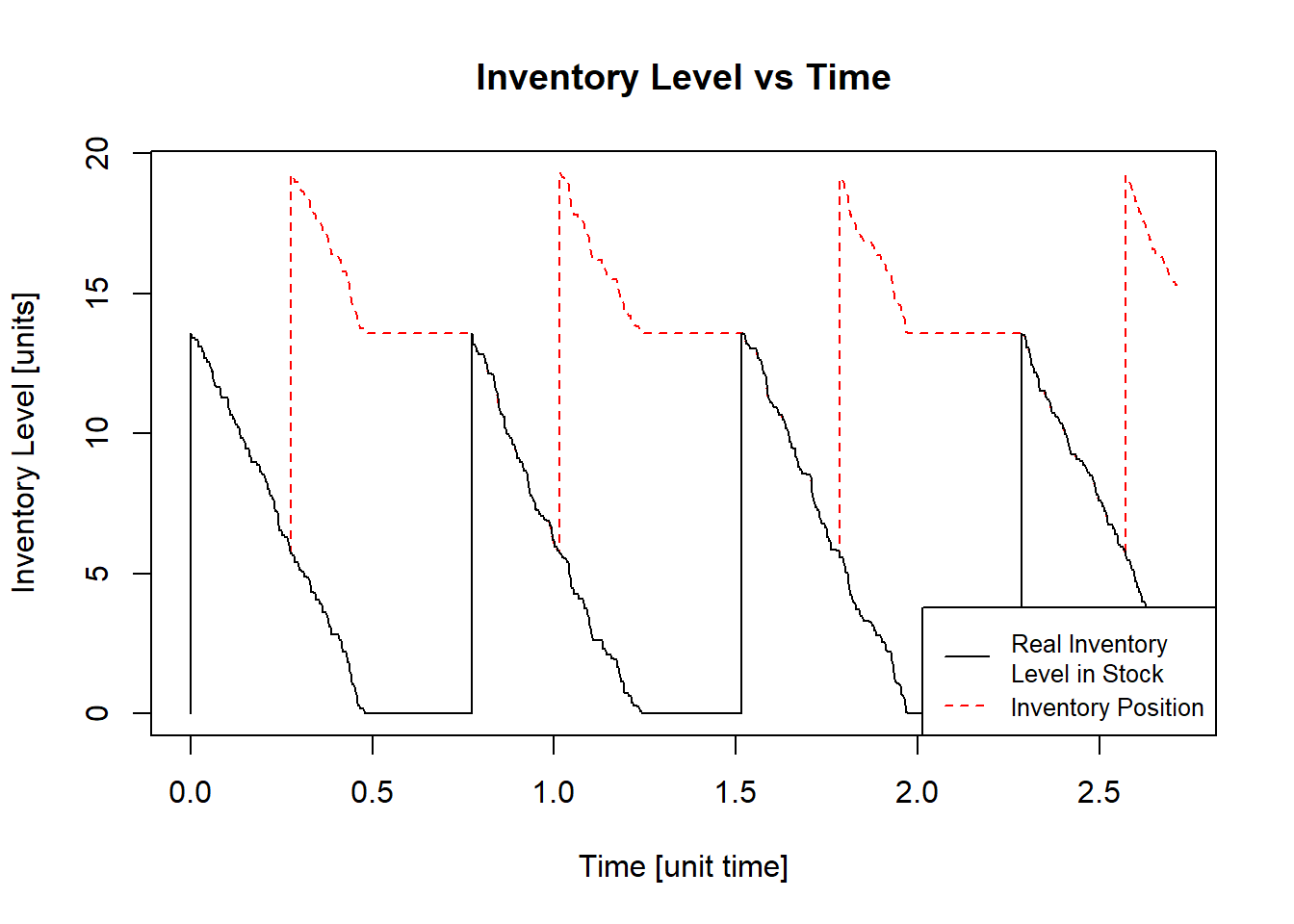
This result means that the metallurgy should order \(13.56\ kg\) once \(5.77\ kg\) or less are available in the stock. The orders are placed approximately every \(1.36\ months\) or (in a month with 30 days) \(40.8\ days\).
5.1.1.2 QR Model: Poisson Distribution Demand
5.1.1.2.1 Theory
When the demand has a behavior of a Poisson Distribution, it has a mean \(\lambda \left[\frac{units}{time}\right]\) (Koehrsen (2019)).
Following the steps in Chapter 5.1.1, with a Poisson Distribution Demand, a mean \(\lambda\), an order cost \(K \left[\frac{\$}{order}\right]\), a holding cost \(h \left[\frac{\$}{unit*time}\right]\), a cost per missing unit \(p \left[\frac{\$}{missing\ unit}\right]\), and a unit cost \(c \left[\frac{\$}{unit}\right]\):
- Initially: \(Q_1 = \sqrt{\frac{2K\lambda}{h}}\)
- Backorders system: \(R = inv.Pois.Dist\left(1 - \frac{Qh}{p\lambda}, mean = \lambda\right)\)
- Lost Sales system: \(R = inv.Pois.Dist\left(1 - \frac{Qh}{Qh+p\lambda}, mean = \lambda\right)\)
- To find de shortages expected value \(n(R)\) with a poisson distribution, since it is a discrete distribution, the Equation (5.3) will be a summation: \[\sum_{x_\tau = R}^{\infty}{(x_\tau - R)f(x_\tau)}\] Where \(x_\tau\) is the demand in the Lead Time \(\tau\) period. \(f(x_\tau)\) must be calculated with \(\lambda_\tau = \lambda\tau\). The simplest way to calculate this summation is making a loop until the sum doesn’t change, with higher \(x\) after \(\lambda\), \(f(x)\) will be smaller, as shown in Figure 5.2
- Now, \(Q = \sqrt{\frac{2\lambda\left(K+pn(R)\right)}{h}}\).
- Steps 2 to 4 should be repeated until \(Q\) and \(R\) converge.
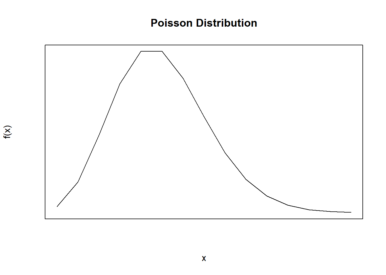
Figure 5.2: Poisson Distribution
5.1.1.2.2 Using InvControl Package qrPoisson(m,k,c,h,p,t,b)
The InvControl Package has the function qrPoisson(m,k,c,h,p,t,b). The parameters for this function are:
- m is the mean of the demand \(\lambda \left[\frac{units}{time}\right]\).
- k is the ordering cost \(K \left[\frac{\$}{order}\right]\).
- c is the purchase cost \(c \left[\frac{\$}{unit}\right]\)
- h is the holding cost \(h \left[\frac{\$}{time*unit}\right]\).
- p is the shortage cost per missing unit \(p \left[\frac{\$}{unit\ missing}\right]\).
- t is the Lead Time period \(\tau [time]\).
- b is TRUE when the system allows Backordes and FALSE when the system manage Lost Sales.
Suppose a cellphone store where is expected to have 5 customers who buy a smartphone each one in a day. The costs associated to ordering, purchase every unit, holding on inventory, and missing unit are \(k = \frac{\$1245}{order}\), \(c = \frac{\$439}{smartphone}\), \(h = \frac{\$1}{smartphone*day}\), and \(p = \frac{\$50}{smartphone\ missing}\), respectively. This company has a system that can check the inventory level all the time, backorders are allowed and the orders take \(3\ days\) to arrive. The function qrPoisson(m,s,k,c,h,p,t,b) shows the optimal reorder point \(R\) and the optimal order quantity \(Q\):
library(invControl)
m = 5
k = 1245
c = 439
h = 1
p = 50
t = 3
b = TRUE
result = qrPoisson(m, k, c, h, p, t, b)
## [1] "Optimal Order Quantity - Q* = 115"
## [1] "Reorder Point - R = 15"
## [1] "Total Average Cost (per time unit) - G(Q) = $ 2309.97"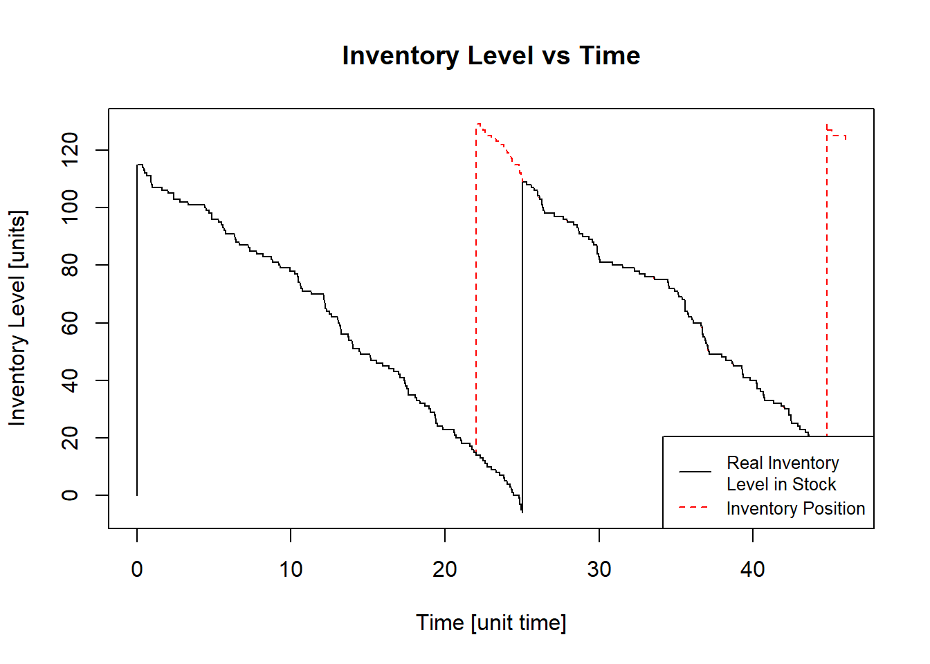
This result means that the cellphone store should order \(115\ smartphones\) once \(15\ smartphones\) or less are available in the stock. The orders are placed approximately every \(23\ days\).