Chapter 4 Inventory Models with Deterministic Demand
Following the two main criteria described in Chapters 2 and 3, there are different inventory models that can be adjusted form standard to modified situations.
As mentioned in the Chapter 2, there are two main types of demand: Deterministic and Stochastic. For cases with deterministic demand, due to it is known, the revision system is not relevant in the different models explained in this section. When the demand has no uncertainty, the inventory level is not expected to vary as projected. The next inventory models for deterministic demand and continuous or periodic revision system are:
4.1 Economic Order Quantity (EOQ)
The EOQ model determines an optimal order quantity seeking minimize the total cost related to order, purchase and holding the inventory. This model calculates the optimal order quantity (\(Q^*\)) based on the average total cost related to the costs mentioned above:
- Setup cost \(K\): it is the money paid every time an order is placed.
- Acquisition cost (unit cost) \(c\): it is the money paid for every unit purchased.
- Holding cost \(h\): it is the money paid per unit every unit of time used (this would be days, weeks, months, years, etc.). This holding cost can be calculated based on a rate \(i\) of the unit cost \(c\): \(h = i*c\).
The average total cost is calculated as follows:
\[\begin{equation} G(Q) = \frac{K}{T} + \frac{cQ}{T} + h\overline{I} \tag{4.1} \end{equation}\]
The first term \(\frac{K}{T}\) refers to the total ordering cost in a given period of time. Generally, this period of time is one year, but it can be used in months, weeks or days. This cost is calculated by dividing the setup cost \(K\) by the time in a cycle \(T\). A cycle starts when an order is placed.
The second term \(\frac{cQ}{T}\) refers to the total cost for a whole order. When an order is placed, \(Q\) units are ordered. Since an order is placed every \(T\) (time in a cycle), this term is calculated by dividing the total cost of purchase \(cQ\) by the time in cycle \(T\).
The third term \(h\overline{I}\) refers to the average holding cost. This is calculated by multiplying \(h\) (holding cost per unit) by the average inventory \(\overline{I}\). The average inventory is calculated as follows:
\[\begin{equation} \overline{I} = \frac{\int_0^T I(t)\,dt}{T} \tag{4.2} \end{equation}\]
Where \(I(t)\) is the inventory level behavior over time and \(T\) is the time in a cycle.
Depending on the expected behavior of the inventory level and the demand conditions, different cases may arise:
4.1.1 EOQ Classic
4.1.1.1 Theory
In the classic model, the demand rate is expected to be the same for the whole time horizon, it means that the demand rate will not change in any part of the cycle \(T\). The Figure 4.1 shows this demand behavior.
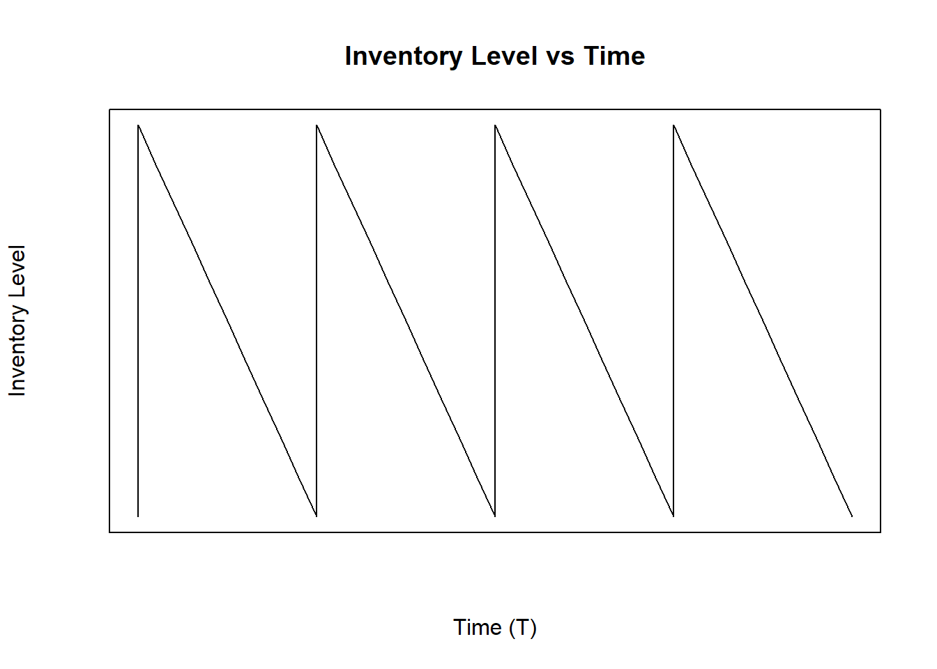
Figure 4.1: Inventory Level with Constant Demand Rate
As mentioned above, the EOQ model seeks to get an optimal \(Q^*\) to minimize the average total cost \(G(Q)\). To solve the EOQ problem, it is necessary to find the optimal quantity that should be ordered in pursuit of the minimum cost \(G(Q)\). Using a constant demand rate \(\lambda\), constant order cost \(K\), constant holding cost per unit \(h\), and no time between the time an order is placed and its arrival is 0 (\(LeadTime (\tau) = 0\)), the following conditions can be assumed:
Considering a constant demand rate, the cycle time \(T\) would be the order quantity \(Q\) over the demand rate \(\lambda\): \[T = \frac{Q}{\lambda}\]
The average inventory is defined by the Equation (4.2). With a constant demand rate \(\lambda\), the average inventory will be the division between the area of a triangle and the cycle time \(T\). The area would be calculated multiplying the height (in this case \(Q\)) and the weight (in this case \(T\)), and then divide by 2:
\[\overline{I} = \frac{A}{T} = \frac{\frac{QT}{2}}{T} = \frac{Q}{2}\]
Now, based on the Equation (4.1), the average total cost can be expressed only in terms of \(Q\) as follows:
\[\begin{equation} G(Q) = \frac{K\lambda}{Q} + c\lambda + \frac{hQ}{2} \tag{4.3} \end{equation}\]
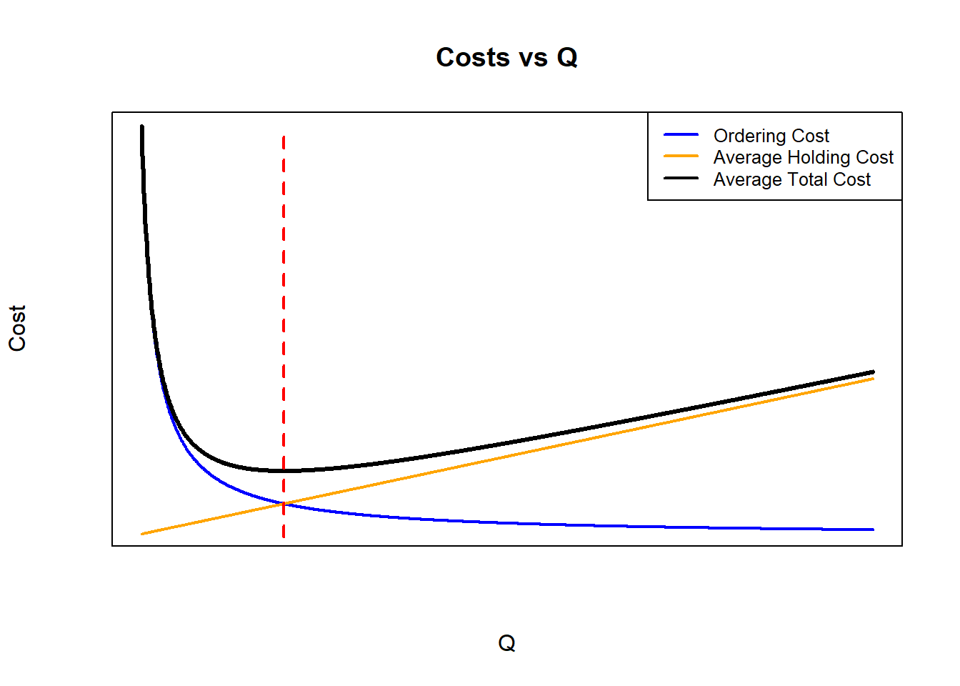
Figure 4.2: Average Total Cost, Average Holding Cost and Ordering Cost vs Q
In the Figure 4.2, the ordering, holding and average total costs are plotted with different values of \(Q\). With the equation (4.3), the total cost for purchasing when ordered \((c\lambda)\) will be always the same, regardless of the value of Q, this is why the average total cost (black line) can be only the sum of the holding cost and ordering cost for comparison purposes (Cargal (n.a.)). As can be seen, the average total cost is a convex curve, with an optimal economic order quantity which value gets the minimum cost. For this reason, to get optimal EOQ \(Q^*\), the derivative of the average total cost function \(G(Q)\) must be equal to \(0\):
\[\frac{dG(Q)}{dQ} = 0\] \[\frac{dG(Q)}{dQ} = -\frac{K\lambda}{Q^2} + \frac{h}{2} = 0\] \[\frac{K\lambda}{Q^2} = \frac{h}{2}\] From the last equation, it can be seen that if the holding and ordering costs are equalized, it is also possible to get the optimal EOQ \(Q^*\). As shown in the Figure 4.2, the red dashed line is above the \(Q^*\), showing that when those costs are equal, the \(Q^*\) can be cleared.
Finally, the optimal EOQ \(Q^*\) would be:
\[\begin{equation} Q^* = \sqrt{\frac{2K\lambda}{h}} \tag{4.4} \end{equation}\]
4.1.1.2 Using InvControl Package EOQ_const(d,k,h,c)
The InvControl Package has the function EOQ_const(d,k,h,c). The parameters for this function are:
- d is the constant demand rate \(\lambda \left[\frac{units}{time}\right]\).
- k is the ordering cost \(K \left[\frac{\$}{order}\right]\).
- h is the holding cost \(h \left[\frac{\$}{time*unit}\right]\).
- c is the purchase cost \(c \left[\frac{\$}{unit}\right]\)
Suppose there is a company that sells computers. The owner wants to know when they should order more computers to hold in stock and how many of them should be purchased. Each order costs to the company \(\$500.00\), purchase each computer costs \(\$345.00\), and hold one computer every month costs \(\$15.00\). In addition, they have an estimated rate of monthly demand of \(498 \frac{units}{month}\). The function EOQ_const(d,k,h,c) shows the optimal EOQ \(Q^*\) as follows:
library(invControl)
d = 498
k = 500.00
h = 15.00
c = 345.00
Q = EOQ_const(d,k,h,c)
## [1] "Economic Order Quantity - Q* = 182.21"
## [1] "Cycle Time - T = 0.37"
## [1] "Total Average Cost (per time unit) - G(Q) = $ 174543.13"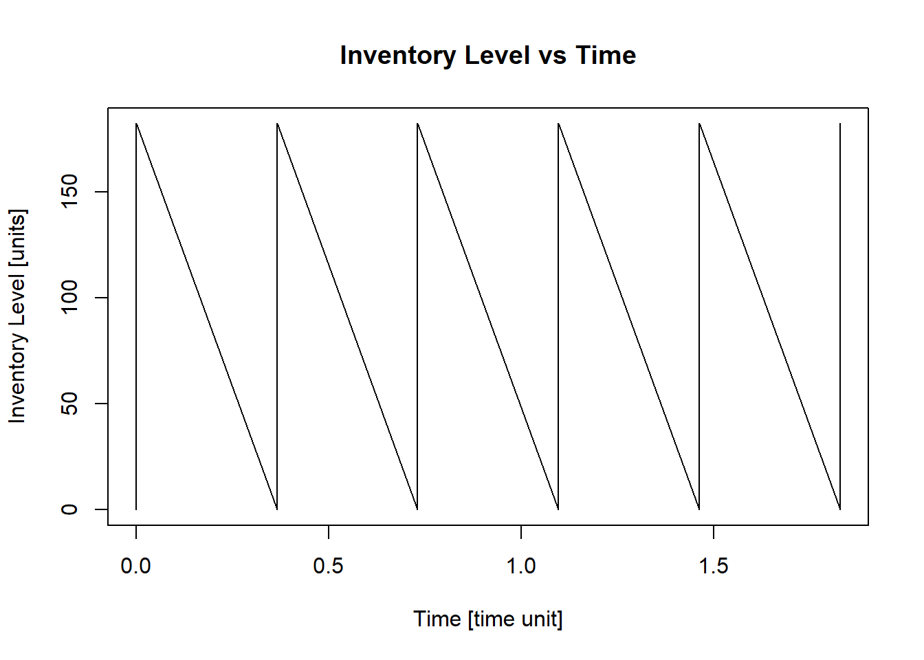
This result means that the owner should order \(182\ computers\) every \(0.37\ months\) or approximately every \(11\ days\) in a month of \(30\) days.
4.1.2 EOQ No Constant Demand in A Cycle
4.1.2.1 Theory
As a modified model of the EOQ Classic from Chapter @ref(eoq_classic), some cases can have a no constant demand in each cycle. For an EOQ model with no constant demand in a cycle, it is necessary to get the economic order quantity \(Q^*\) based on the Equation (4.1):
\[\begin{equation} G(Q) = \frac{K}{T} + \frac{cQ}{T} + h\overline{I} \end{equation}\]
In a situation when the cycle does not have a constant demand, the inventory level plot looks life Figure 4.3.
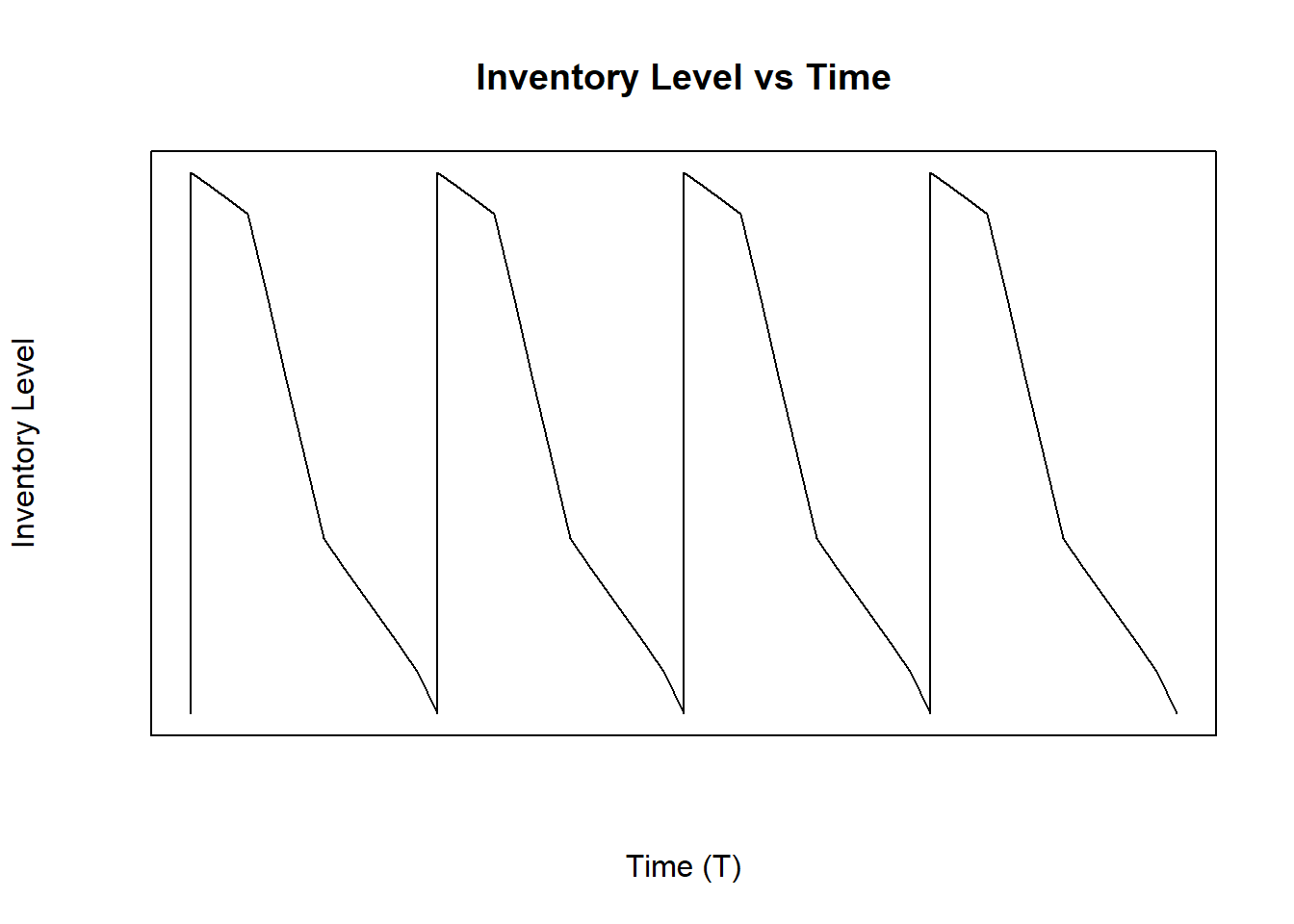
Figure 4.3: Inventory Level With No Constant Demand Rate in a Cycle
Since there is no constant demand and a cycle can have different demand rates, the average inventory will change and the assumptions made with EOQ classic (Chapter @ref(eoq_classic)) can not be used in this modified case. It means that \(\overline{I} \neq \frac{Q}{2}\) and \(\lambda \neq \frac{Q}{T}\), because there are different demand rates. In a cycle can be multiple different demand rates in a part of the cycle. To model this situation, the cycle must be separated in the different portions of the demand.
There are \(n\) different demand rates in the cycle, each demand rate will be held in one portion of the cycle, that is, the cycle will be divided into \(n\) portions, not necessarily all equal:
\[Demand\ Rates\ in\ a\ Cycle = \left[\lambda_1, \lambda_2, \lambda_3,...,\lambda_n\right]\] \[Portions\ of\ the\ Cycle =\left[t_1, t_2, t_3,...,t_n\right]\] \[\sum_{i=1}^{n}{t_i}=1\]
Since there are multiple demand rates, the cycle time \(T\) and average inventory will be the following:
\[T=\frac{Q}{\sum_{i=1}^{n}{t_i \lambda_i}}\] \[\overline{I} = \left[ \frac{\sum_{i=1}^{n}{t_i^2 \lambda_i}}{2} + \sum_{i=2}^{n}{\left(t_i\lambda_i*\sum_{j=1}^{i-1}{t_j}\right)} \right]*T = \frac{\left[ \frac{\sum_{i=1}^{n}{t_i^2 \lambda_i}}{2} + \sum_{i=2}^{n}{\left(t_i\lambda_i*\sum_{j=1}^{i-1}{t_j}\right)} \right]*Q}{\sum_{i=1}^{n}{t_i \lambda_i}}\]
Based on the Equation (4.1), the average total cost for a model with multiple demand rates in a cycle in terms only of \(Q\) will be:
\[\begin{equation} G(Q) = K\frac{\sum_{i=1}^{n}{t_i \lambda_i}}{Q}+c\sum_{i=1}^{n}{t_i \lambda_i}+h\frac{\left[ \frac{\sum_{i=1}^{n}{t_i^2 \lambda_i}}{2} + \sum_{i=2}^{n}{\left(t_i\lambda_i*\sum_{j=1}^{i-1}{t_j}\right)} \right]*Q}{\sum_{i=1}^{n}{t_i \lambda_i}} \tag{4.5} \end{equation}\]
Due to the fact that the purchase total cost is constant independent of the value of Q, as shown in the Figure 4.2, the minimum total cost will be when \(\frac{dG(Q)}{dQ}=0\). Thus, after performing the derivative of the total cost \(G(Q)\) with respect to \(Q\), the economic order quantity \(Q^*\) will be:
\[\begin{equation} Q^*=\sqrt{\frac{K\left(\sum_{i=1}^{n}{t_i \lambda_i}\right)^2}{h\left[ \frac{\sum_{i=1}^{n}{t_i^2 \lambda_i}}{2} + \sum_{i=2}^{n}{\left(t_i\lambda_i*\sum_{j=1}^{i-1}{t_j}\right)} \right]}} \tag{4.6} \end{equation}\]
4.1.2.2 Using InvControl Package EOQ_ncd(n,d,t,k,h,c)
The InvControl Package has the function EOQ_ncd(n,d,t,k,h,c). The parameters for this function are:
- n is the number of different demand rates \(\lambda_i\) in a cycle.
- d is the vector of demand rates \(\{\lambda_1,\lambda_2, \lambda_3,...,\lambda_n\} \left[\frac{units}{time}\right]\).
- t is the vector of the portion or percentage of the cycle for each demand \(\{t_1,t_2,t_3,...,t_n\}\).
- k is the ordering cost \(K \left[\frac{\$}{order}\right]\).
- h is the holding cost \(h \left[\frac{\$}{time*unit}\right]\).
- c is the purchase cost \(c \left[\frac{\$}{unit}\right]\)
Suppose there is a fashion company which is planning to release a different collection periodically and wants to know how many items should order from every collection. However, for each collection, the demand behavior has different rates in the cycle. Once the collection is released, the demand is \(500 \frac{units}{month}\) in the \(45\%\) of the length of the collection. After that, the demand goes down to \(250 \frac{units}{month}\) in the \(20\%\) of the length of the collection. Then, in the next \(5\%\) of the collection length, the fashion company does not have demand at all. Finally, the fashion company offers discounts on clothing and the demand goes a little higher to \(348 \frac{units}{month}\) in the remaining time of the collection. Every order costs \(\$1,240.00\), every unit costs \(\$152.00\), and the holding cost for each item every month is \(\$55.49\). The function EOQ_ncd(n,d,t,k,h,c) shows the optimal EOQ \(Q^*\) as follows:
library(invControl)
n = 4
d = c(500,250,0,348)
t = c(0.45,0.20,0.05,0.30)
k = 1240.00
h = 55.49
c = 152.00
Q = EOQ_ncd(n,d,t,k,h,c)
## [1] "Economic Order Quantity - Q* = 119.38"
## [1] "Cycle Time - T = 0.31"
## [1] "Total Average Cost (per time unit) - G(Q) = $ 65550.13"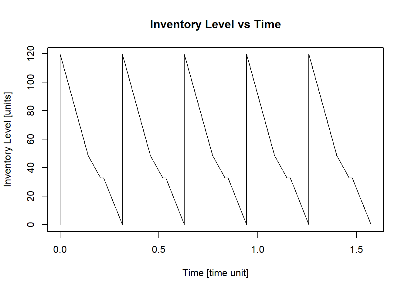
This result means that the fashion company should order \(119\ items\) from a new collection every \(0.31\ months\) or approximately every \(9\ days\) in a month of \(30\) days.
4.1.3 EOQ with Different Demand Rates in a Time of Cycle Known
4.1.3.1 Theory
Some companies can have seasonal demand rates in a known time, for example, a company of winter clothes will have high demand at the end and at the beginning of the year, but low (or lower) demand during the middle of the year. In this situation, the cycle time \(T\) will be 12 months and the different times in the cycle would be determined by the company based on the different demand rates in the year.
With this modified model, the different demand rates \(\lambda_i\) are known as well as the individual cycles \(t_i\) in the cycle time \(T = \sum{t_i}\). The purpose of this EOQ modified model is to calculate a economic order quantity to be ordered every time the inventory level \(I\) reaches \(0\) units, no matters the demand rate \(\lambda_i\) at the moment of the order; it means, the same quantity \(Q^*\) will be ordered every time is needed.
In accordance with the Equation (4.1), the average total cost will be the following:
\[\begin{equation} G(Q) = m\frac{K}{T} + m\frac{cQ}{T} + h\overline{I} \tag{4.7} \end{equation}\]
Where \(m\) is the number of times an order was placed. In this case, considering the cycle time \(T\) is known, the only unknown factors in the Equation (4.7) are \(Q\) (the EOQ to be calculated) and \(\overline{I}\) (the average inventory in cycle time \(T\)). This modified model must follow the next rules:
- The number of times an order is placed in a cycle time \(T\) (\(m\)) must be a positive whole number: \(m \in \mathbb{N}\). \(m\) is calculated based on the total demand \(D = \sum_{i=1}^n{\left(\lambda_it_i\right)}\) in the cycle time \(T\) divided by \(Q\):
\[m = \frac{D}{Q} = \frac{\sum_{i=1}^n{\left(\lambda_it_i\right)}}{Q} \in \mathbb{N}\]
- At the beginning of the cycle time \(T\), the inventory level must be equal to the order quantity \(Q\), and at the end must be equal to \(0\). Making sure that \(m\) is a positive whole number, this fact is fulfilled by default.
- No backorders are allowed. This means, if a customer wants to buy an item, and there is no availability, the sale will not be completed.
- Lead time \(\tau\), time between the moment an order is placed and it arrives, is equal to \(0\).
The Figure 4.4 shows how the inventory level will look through time with this modified model, where only one cycle time \(T\) is shown:
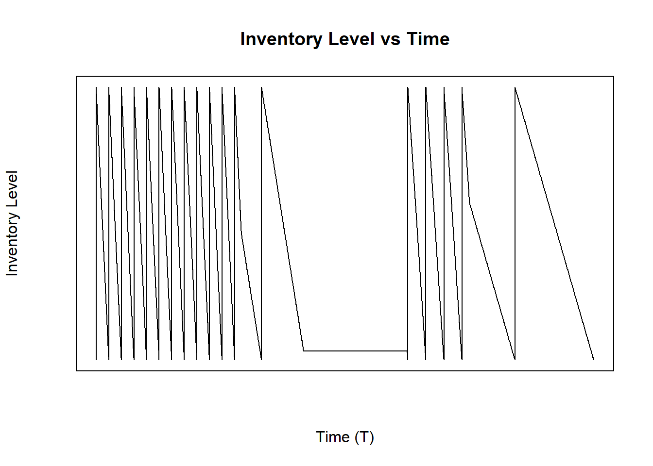
Figure 4.4: Inventory Level With Different Demand Rates in a Time of Cycle Known
The average inventory \(\overline{I}\) is calculated based on the whole cycle time \(T\) as follows:
Notes: (Hein (2003))
- The notation \(\lceil{x}\rceil\) is the ceiling function of \(x\). This function sets \(\lceil{x}\rceil\) to the closest integer greater than or equal to \(x\). For example, \(\lceil{1.84}\rceil = 2\) or \(\lceil{2.15}\rceil = 3\).
- The notation \(\lfloor{x}\rfloor\) is the floor function of \(x\). This function sets \(\lfloor{x}\rfloor\) to the closest integer less than or equal to \(x\). For example, \(\lfloor{5.46}\rfloor = 5\) or \(\lfloor{8.99}\rfloor = 8\).
As shown in the Equation (4.2), the average inventory \(\overline{I}\) is calculated with the integral from \(0\) to \(T\) of the function of inventory level through time. In this case, the integral \(\int_0^T I(t)\) is the area under the plot shown in Figure 4.4. Since this area is not like the models in Chapters 4.1.1 and 4.1.2, it is better to divide the whole area in two: \(A_1\) will be the area under the first demand rate and \(A_2\) will be the area under the others demand rates:
\[\begin{equation*} A_1 = \begin{cases} Qt_1-\bigg\lfloor{\frac{\lambda_1t_1}{Q}}\bigg\rfloor\frac{Q^2}{2\lambda_1}-\left(t_1-\bigg\lfloor{\frac{\lambda_1t_1}{Q}}\bigg\rfloor\frac{Q}{\lambda_1}\right)^2\frac{\lambda_1}{2} & \mbox{if }\lambda_1>0 \\ Qt_1 & \mbox{if }\lambda_1=0 \end{cases} \end{equation*}\]
For the second area, it is important to know what is the inventory level at the moment a new demand rate will start, this inventory level \(x\) is calculated as follows:
\[x_i = \Bigg\lceil\frac{\sum_{j = 1}^{i-1}{\lambda_jt_j}}{Q}\Bigg\rceil Q - \sum_{j = 1}^{i-1}{\lambda_jt_j}\]
However, it is possible that \(x_i\) is exactly equal to \(0\), in this case, \(x_i = Q\):
\[\begin{equation*} x_i = \begin{cases} x_i & \mbox{if }x_i>0 \\ Q & \mbox{if }x_i=0 \end{cases} \end{equation*}\]
After knowing the inventory level at the moment the new demand rate will start, the second area can be calculated; however, it is necessary to define two additional sub-areas \(A_{i_1}\) and \(A_{i_2}\):
\[A_{i_1} = \min{\left(t_i,\frac{x_i}{\lambda_i}\right)}x_i -\left(\min{\left(t_i,\frac{x_i}{\lambda_i}\right)}\right)^2\frac{\lambda_i}{2}\]
\[A_{i_2} = Q\left(t_i-\min{\left(t_i,\frac{x_i}{\lambda_i}\right)}\right) - \Bigg\lfloor{\frac{\lambda_i\left(t_i-\min{\left(t_i,\frac{x_i}{\lambda_i}\right)}\right)}{Q}}\Bigg\rfloor \frac{Q^2}{2\lambda_i}-\left(t_i-\min{\left(t_i,\frac{x_i}{\lambda_i}\right)}-\Bigg\lfloor{\frac{\lambda_i\left(t_i-\min{\left(t_i,\frac{x_i}{\lambda_i}\right)}\right)}{Q}}\Bigg\rfloor \frac{Q}{\lambda_i}\right)^2 \frac{\lambda_i}{2}\]
\[\begin{equation*} A_i = \begin{cases} A_{i_1} + A_{i_2} & \mbox{if }\lambda_i>0 \\ x_i t_i & \mbox{if }\lambda_i=0 \end{cases} \end{equation*}\]
Now, the second area will be:
\[A_2 = \sum_{i = 2}^{n}{A_i}\]
In this way, the average inventory is:
\[\overline{I} = \frac{A_1+A_2}{T}\]
As it can be observed, the whole equation \(G(Q)\) is hard to derive with respect to \(Q\) due to the multiple conditions the average inventory has. For this reason, an approximation to the optimal EOQ \(Q^*\) can be calculated with iterations between \(0.01\) and \(D\).
4.1.3.2 Using InvControl Package EOQ_tknown(n,d,t,k,h,c)
The InvControl Package has the function EOQ_tknown(n,d,t,k,h,c). The parameters for this function are:
- n is the number of different demand rates \(\lambda_i\) in a cycle.
- d is the vector of demand rates \(\{\lambda_1,\lambda_2, \lambda_3,...,\lambda_n\} \left[\frac{units}{time}\right]\).
- t is the vector of different times in a cycle T for each demand rate \(\{t_1,t_2,t_3,...,t_n\}[time]\).
- k is the ordering cost \(K \left[\frac{\$}{order}\right]\).
- h is the holding cost \(h \left[\frac{\$}{time*unit}\right]\).
- c is the purchase cost \(c \left[\frac{\$}{unit}\right]\)
Suppose there is a winter clothes company. This company will have the highest demand rate at the end and beginning of the year, due to the winter season. However, in the rest of the year, some people buy winter staff because it is cheaper, for example, in June or July than in December or January. The company has found the demand rates similar all the years and they are the following:
- November, December, January and February: \(8405 \frac{units}{month}\)
- March and April: \(3522 \frac{units}{month}\)
- May, June, July, August and September: \(985 \frac{units}{month}\)
- October: \(2500 \frac{units}{month}\)
Each unit bought by the company has a cost of \(\$79.99\), each delivery has a cost of \(\$250.00\), and the holding cost is \(\$12.00/(unit*month)\). The function EOQ_tknown(n,d,t,k,h,c) shows an approximation of the optimal EOQ \(Q^*\) as follows:
library(invControl)
n = 4
d = c(8405,3522,985,2500)
t = c(4,2,5,1)
k = 250.00
h = 12.00
c = 79.99
Q = EOQ_tknown(n,d,t,k,h,c)
## [1] "Economic Order Quantity - Q* = 2531"
## [1] "Total Average Cost (per time unit) - G(Q) = $ 335906.5"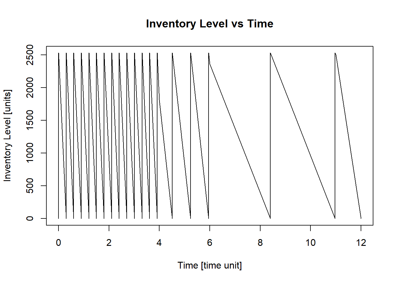
This result means that the winter clothes company should order \(2531\) units every time there is no stock. the resulting plot of the function shows in which months an order should be placed, where \(0\) in the x-axis means the beginning of the month of November.