Value-at-Risk and Expected Shortfall
Question
We consider the daily losses on a position in a particular stock. The current value of the position is \(V_t = 10,000\). The loss process for this portfolio is defined as \[ L^{\Delta}_{t+1} = -V_t \omega_t^\prime X_{t+1}, \] where \(X_{t+1}\) represents the daily log-returns of the stock. We assume that \(X_{t+1}\) has mean zero and standard deviation \(\sigma = \frac{0.2}{\sqrt{250}}\), i.e. we assume an annualised volatility of \(20\%\).
We compare two different models for the distribution of \(X_{t+1}\):
A normal distribution; and
A \(t\)-distribution with \(\nu=4\) degrees of freedom, scaled to have standard deviation \(\sigma\).
- For a standard \(t\)-distribution \(t(\nu, 0, 1)\), the variance is \(\frac{\nu}{\nu-2}\).
- The \(t\)-distribution is symmetric but has heavier tails than the normal distribution, so that large absolute values are more probable. Empirical studies often find that such heavy-tailed distributions provide a better fit to financial return data.
Questions:
Evaluate and present, in a table, the Value at Risk \(\text{VaR}_\alpha\) and the Expected Shortfall \(\text{ES}_\alpha\) for both models and for various values of \(\alpha \in (0.9,1)\).
Compare your \(\text{VaR}_\alpha\) with \(\text{ES}_\alpha\) by finding the ratio \(\text{VaR}_\alpha / \text{ES}_\alpha\). What findings/conclusions can you draw from your comparisons?
Solution and Code
Start with a clean workspace
Before running your script, it is good practice to remove all existing objects from memory to ensure reproducibility. The command ls() lists all objects in your workspace, and rm() removes them.
This way the workspace is empty and everything you create is clearly visible.
Load required packages
The functions used in this session are available in the QRM and qrmtools packages — comprehensive toolkits for quantitative risk management.
When it comes down to R packages:
install.packages("package"), installs a given package.library("package")loads the package.
Define parameters
Define a set of quantile probabilities \(p\) and the corresponding \(alpha\)-type probabilities for the upper tail. Both sets are vectors.
Next, define the portfolio value, daily standard deviation and degrees of freedom for the \(t\)-distribution.
Compute Value-at-Risk (VaR)
Normal distribution
The quantile function qnorm() gives the quantile at each probability level.
Alternatively, using the upper-tail probabilities:
Both approaches produce the same result.
We get the same results using the (upper tail) alpha vector if we specify lower.tail=FALSE.
Student’s \(t\) distribution
For the \(t\)-distribution, the quantiles are obtained with qt().
Because the variance of a standard t distribution is \(\frac{\nu}{\nu-2}\), we scale by \(\sqrt{\frac{\nu-2}{\nu}}\) to match the same standard deviation as the normal model.
## [1]  137.1341  190.6782  248.3328  335.1372
## [5]  411.8028  641.5889 1165.7670 2086.8939
## [9] 3718.8363
Note: in the QRM package, this can be done by calling the qst function. See ?qst for full details.
## [1]  137.1341  190.6782  248.3328  335.1372
## [5]  411.8028  641.5889 1165.7670 2086.8939
## [9] 3718.8363
Compute Expected Shortfall (ES)
Normal distribution
The expected shortfall under normality can be obtained using ESnorm(), which computes
\[ \text{ES}_\alpha = \sigma \frac{\phi(z_\alpha)}{1-p},\]
where \(z_\alpha = \Phi^{-1}(p)\) and \(\phi\) denotes the standard normal density.
The function ESnorm returns the expected loss given a loss exceeding p under normality, scaled by sigma. The expected loss is calculated by integrating over the tail of the normal distribution, dividing by its length and multiplying by sigma: sd * dnorm(qnorm(p))/(1 - p). See ?ESnorm for full details.
Compute and compare ratios
We next compare tail risk severity using the shortfall-to-quantile ratio: \[ \frac{\text{ES}_\alpha}{\text{VaR}_\alpha}. \] This ratio tends to \(1\) for light-tailed distributions and exceeds \(1\) for heavy-tailed ones.
## [1] 1.369421 1.254040 1.192778 1.145665 1.122725
## [6] 1.089591 1.064389 1.050140 1.041004## [1] 1.630140 1.502392 1.438371 1.393290 1.373740
## [6] 1.350338 1.338540 1.334964 1.333847Summarise and visualise results
Combine all results into one table for easy comparison:
summary <- cbind(p, VaR.normal, VaR.t4, ES.normal, ES.t4, Ratio.normal, Ratio.t4)
colnames(summary) <- c("p", "VaR.normal", "VaR.t4", "ES.normal", "ES.t4",
                       "Ratio.normal", "Ratio.t4")
print(round(summary, 4))
## p VaR.normal VaR.t4 ES.normal
## [1,] 0.9000 162.1049 137.1341 221.9898
## [2,] 0.9500 208.0594 190.6782 260.9148
## [3,] 0.9750 247.9180 248.3328 295.7113
## [4,] 0.9900 294.2623 335.1372 337.1259
## [5,] 0.9950 325.8195 411.8028 365.8058
## [6,] 0.9990 390.8869 641.5889 425.9069
## [7,] 0.9999 470.4225 1165.7670 500.7125
## [8,] 1.0000 539.4708 2086.8939 566.5199
## [9,] 1.0000 601.2659 3718.8363 625.9201
## ES.t4 Ratio.normal Ratio.t4
## [1,] 223.5478 1.3694 1.6301
## [2,] 286.4734 1.2540 1.5024
## [3,] 357.1946 1.1928 1.4384
## [4,] 466.9432 1.1457 1.3933
## [5,] 565.7101 1.1227 1.3737
## [6,] 866.3618 1.0896 1.3503
## [7,] 1560.4264 1.0644 1.3385
## [8,] 2785.9275 1.0501 1.3350
## [9,] 4960.3597 1.0410 1.3338Plot the VaR and ES for both models:
plot(p, VaR.normal, type = "o", ylim = range(summary[, 2:5]),
     ylab = "Value (£)", xlab = "Confidence level (p)")
title("VaR and ES")
lines(p, VaR.t4, type = "o", col = 2)
lines(p, ES.normal, type = "o", col = 3)
lines(p, ES.t4, type = "o", col = 4)
legend("topleft",
       legend = c("VaR, normal", "VaR, t(4)", "ES, normal", "ES, t(4)"),
       col = 1:4, pch = 1)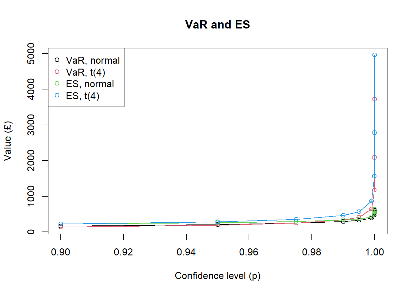
Plot the ES/VaR ratio to highlight differences in tail behaviour:
plot(p, Ratio.normal, type = "o", ylim = range(summary[, 6:7]),
     ylab = "ES / VaR", xlab = "Confidence level (p)")
title("Shortfall-to-Quantile Ratio")
lines(p, Ratio.t4, type = "o", col = 2)
legend("bottomleft",
       legend = c("ES/VaR, normal", "ES/VaR, t(4)"),
col = 1:2, pch = 1) 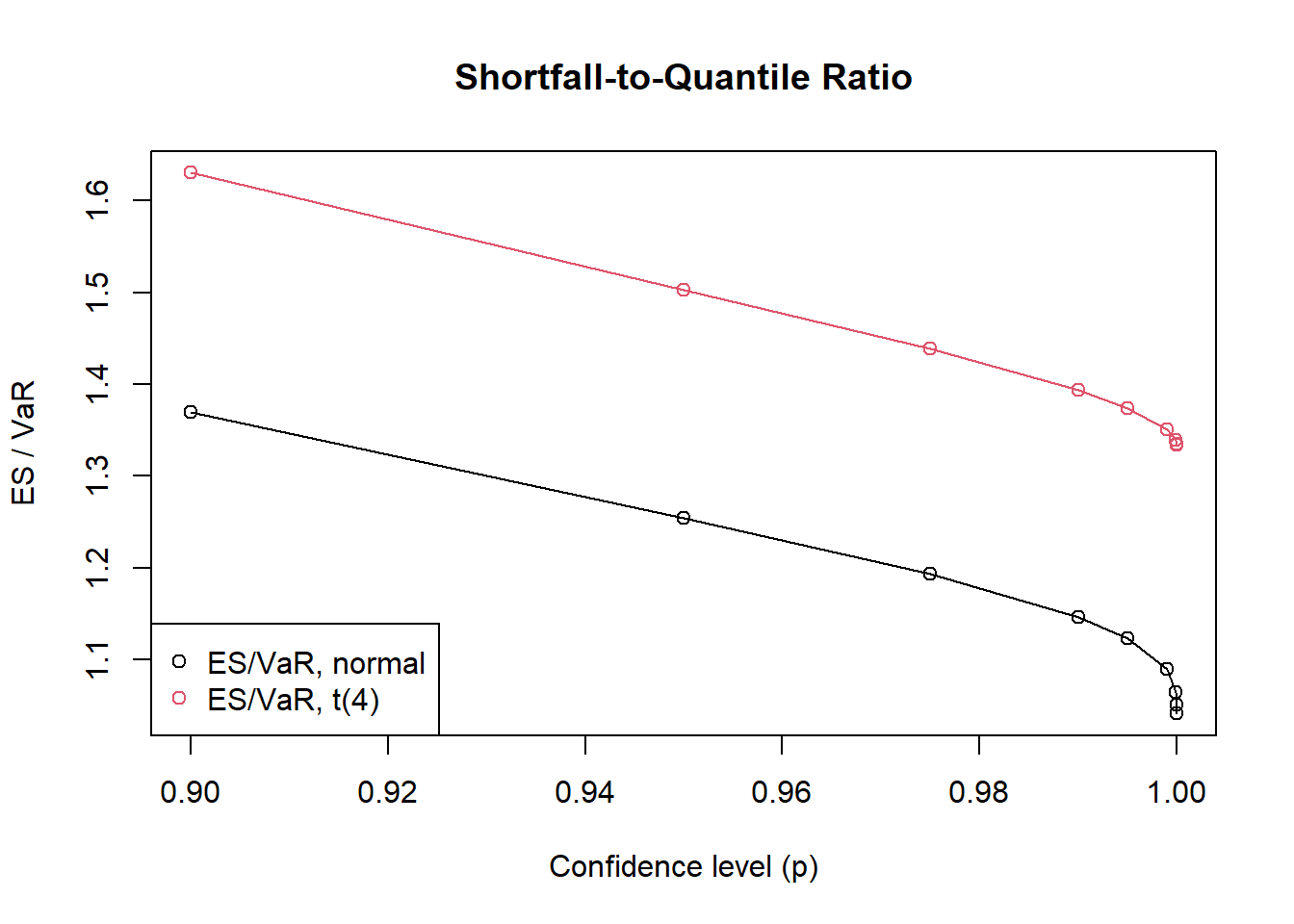
Findings and conclusions
The $Student’s \(t\) model exhibits heavier tails, meaning that extreme losses are more likely compared with the normal model.
At moderate confidence levels (e.g. \(95\%\) or \(97.5\%\)), the difference between the two models is small — the normal model may even appear slightly riskier.
At high confidence levels (above \(99\%\)), the \(t\)-distribution produces noticeably higher VaR and ES values, reflecting greater tail risk.
Expected Shortfall (ES) captures the tail risk more effectively than VaR, as ES continues to increase significantly for the t model even when VaR appears similar.
As \(\alpha \rightarrow 1\): \[ \frac{\text{ES}_\alpha}{\text{VaR}_\alpha} \rightarrow \begin{cases} 1, & \quad\text{Normal distribution}, \\ \nu/(\nu - 1) > 1, & \quad t_\nu \text{ distribution}. \end{cases} \]
This result highlights that for a heavy-tailed distribution, the difference between ES and VaR is more pronounced than that for the normal distribution.