Basic Terminology

Prerequisites

You will need to have both R and RStudio installed on your computer.

• R from https://cran.r-project.org/.

• An integrated development environment (IDE) (e.g., editor, build tools): RStudio: http://www.rstudio.com/.

R (contributed) packages can be installed via either of the following versions.

• Release versions:

  • Comprehensive R Archive Network (CRAN): install.packages(“mypkg”).

  • Bioconductor: devtools::install_bioc(“mypackage”) or BiocManager::install(“mypackage”).

• Development versions:

  • R-Forge: install.packages(“mypkg”, repos = “https://R-Forge.R-project.org”)).

  • GitHub: devtools::install_github(“maintainer/mypkg”).

To work with R,

• create a script (a file, e.g. myscript.R) containing the R source code; and

• run the script interactively by executing it line-by-line.

  To run the current line, press Control+R or right-click and select Run line or selection. If you want to understand a command, enter ?command in R console.

This is good practice: clear all objects from the memory before starting an R session. Just make sure you place the code below as the first line in each of your R scripts.

rm(list=ls(all=TRUE))  

Creating Objects in R

In R, everything is an object — numbers, text, vectors, matrices, and even functions. You can assign values to objects using the assignment operator <-.

Scalars

A scalar is a single value (a number or a piece of text).

scalar1 <- 1 

Run the next line, and the value of the object scalar1 will appear in the R Console.

scalar1 

## [1] 1

You can also create other types of scalars:

scalar2 <- 3.14      # numeric
scalar3 <- "Hello"   # character (text)
scalar4 <- TRUE      # logical (boolean)

To check the type of any object:

typeof(scalar3)

## [1] "character"

Vectors

A vector is a sequence of elements of the same type (numeric, character, or logical).

Creating simple vectors

# Create a numeric vector of length 5, all elements equal to 1
vector1 <- array(1, 5)
vector1

## [1] 1 1 1 1 1

Generating sequences

The : operator and the seq() function can be used to create numerical sequences.

# ':' means 'to'
sequence1 <- 1:10
sequence1

##  [1]  1  2  3  4  5  6  7  8  9 10

# Create a custom sequence
sequence2 <- seq(1, 10, by = 2)
sequence2

## [1] 1 3 5 7 9

# Create a sequence with decimal steps
sequence3 <- seq(1, 10, by = 2)
sequence3

## [1] 1 3 5 7 9

Combining values

# Use c() to combine elements into a vector
sequence4 <- c(1, 4, -7, 10, -20)
sequence4

## [1]   1   4  -7  10 -20

Repeating values

The rep() function allows us to repeat elements or entire sequences.

# Repeat a single value
repeated1 <- rep(5, 2)
repeated1

## [1] 5 5

# Repeat a vector multiple times
repeated.sequence1 <- rep(1:5, 3)
repeated.sequence1

##  [1] 1 2 3 4 5 1 2 3 4 5 1 2 3 4 5

# Repeat each element of a vector
repeated.sequence2 <- rep(1:5, each = 3)
repeated.sequence2

##  [1] 1 1 1 2 2 2 3 3 3 4 4 4 5 5 5

Accessing elements in a vector

You can access elements of a vector using square brackets [].

# Display the 5th element in a vector
sequence1[5]

## [1] 5

# Display the first three elements
sequence1[1:3]

## [1] 1 2 3

# Exclude the second element
sequence1[-2]

## [1]  1  3  4  5  6  7  8  9 10

Useful vector operations

# Add two vectors of the same length
v1 <- 1:5
v2 <- seq(2, 10, by = 2)
v1 + v2

## [1]  3  6  9 12 15

# Apply a mathematical function elementwise
sqrt(v1)

## [1] 1.000000 1.414214 1.732051 2.000000 2.236068

# Logical comparison
v1 > 3

## [1] FALSE FALSE FALSE  TRUE  TRUE

Matrices

A matrix is a two-dimensional array (rows × columns) with elements of the same type.

Creating matrices

# Create a 4x5 matrix containing numbers 1 to 20
matrix1 <- array(1:20, c(4, 5))
matrix1

##      [,1] [,2] [,3] [,4] [,5]
## [1,]    1    5    9   13   17
## [2,]    2    6   10   14   18
## [3,]    3    7   11   15   19
## [4,]    4    8   12   16   20

# Create a 4x6 matrix where all entries are 8
matrix2 <- matrix(8, 4, 6)
matrix2

##      [,1] [,2] [,3] [,4] [,5] [,6]
## [1,]    8    8    8    8    8    8
## [2,]    8    8    8    8    8    8
## [3,]    8    8    8    8    8    8
## [4,]    8    8    8    8    8    8

Checking dimensions

dim(matrix1)

## [1] 4 5

dim(matrix2)

## [1] 4 6

Combine matrices and vectors

# Combine 'matrix1' with 'vector1' as a new row
matrix3 <- rbind(matrix1, vector1)
matrix3

##         [,1] [,2] [,3] [,4] [,5]
##            1    5    9   13   17
##            2    6   10   14   18
##            3    7   11   15   19
##            4    8   12   16   20
## vector1    1    1    1    1    1

# Combine two matrices side by side
matrix4 <- cbind(matrix1, matrix2[, 1])
matrix4

##      [,1] [,2] [,3] [,4] [,5] [,6]
## [1,]    1    5    9   13   17    8
## [2,]    2    6   10   14   18    8
## [3,]    3    7   11   15   19    8
## [4,]    4    8   12   16   20    8

Accessing elements

# Element in 2nd row, 3rd column
matrix3[2, 3]

##    
## 10

# Entire 1st row
matrix3[1, ]

## [1]  1  5  9 13 17

# Entire 4th column
matrix3[, 4]

##                                 vector1 
##      13      14      15      16       1

Matrix operations

# Transpose a matrix
t(matrix1)

##      [,1] [,2] [,3] [,4]
## [1,]    1    2    3    4
## [2,]    5    6    7    8
## [3,]    9   10   11   12
## [4,]   13   14   15   16
## [5,]   17   18   19   20

# Multiply two matrices (compatible dimensions required)
matrixA <- matrix(1:6, nrow = 2)
matrixB <- matrix(7:12, nrow = 3)
matrixA %*% matrixB  # matrix multiplication

##      [,1] [,2]
## [1,]   76  103
## [2,]  100  136

# Elementwise multiplication
matrix1 * 2

##      [,1] [,2] [,3] [,4] [,5]
## [1,]    2   10   18   26   34
## [2,]    4   12   20   28   36
## [3,]    6   14   22   30   38
## [4,]    8   16   24   32   40

Strings

Character data (text) is also a common object type in R. You can store single or multiple strings in a variable and manipulate them easily.

Creating and combining strings

# Create a single string
string1 <- "Hello!"
string1

## [1] "Hello!"

# Combine multiple strings into a vector
string2 <- c(string1, "Happy New Year.")
string2

## [1] "Hello!"          "Happy New Year."

# Combine string1 and string2 with "---" in between
string3 <- paste(string2, collapse = "---") 
string3

## [1] "Hello!---Happy New Year."

Naming rows and columns in a matrix

We can use strings to label matrix dimensions for easier interpretation.

# View current column names
colnames(matrix3)

## NULL

# Assign new column names
labels <- c("A", "B", "C", "D", "E")
colnames(matrix3) <- paste("Column", labels, sep = " ") 
colnames(matrix3)

## [1] "Column A" "Column B" "Column C" "Column D" "Column E"

# Assign row names
rownames(matrix3) <- paste("Row", 1:5, sep = " ") 
rownames(matrix3)

## [1] "Row 1" "Row 2" "Row 3" "Row 4" "Row 5"

Basic Calculations

This section introduces basic mathematical operations in R, including scalar multiplication, transposition, inverse (elementwise), and matrix algebra. You will also learn how to perform both element-by-element operations and true matrix multiplication.

Transpose and scalar multiplication

You can multiply a matrix by a scalar, and you can also take the transpose of a matrix using the t() function.

# Multiply scalar by matrix
scalar1 * matrix3

##       Column A Column B Column C Column D Column E
## Row 1        1        5        9       13       17
## Row 2        2        6       10       14       18
## Row 3        3        7       11       15       19
## Row 4        4        8       12       16       20
## Row 5        1        1        1        1        1

# Transpose of matrix3
t(matrix3)  

##          Row 1 Row 2 Row 3 Row 4 Row 5
## Column A     1     2     3     4     1
## Column B     5     6     7     8     1
## Column C     9    10    11    12     1
## Column D    13    14    15    16     1
## Column E    17    18    19    20     1

Inverse

When you raise a matrix to a negative power using ^-1, R performs the operation elementwise, not as a true matrix inverse.

# Element-wise inverse (not matrix inverse)
matrix3^-1 

##        Column A  Column B   Column C   Column D   Column E
## Row 1 1.0000000 0.2000000 0.11111111 0.07692308 0.05882353
## Row 2 0.5000000 0.1666667 0.10000000 0.07142857 0.05555556
## Row 3 0.3333333 0.1428571 0.09090909 0.06666667 0.05263158
## Row 4 0.2500000 0.1250000 0.08333333 0.06250000 0.05000000
## Row 5 1.0000000 1.0000000 1.00000000 1.00000000 1.00000000

Element-by-element operations

You can perform mathematical functions on all elements of a matrix at once. This is called vectorisation — R automatically applies the function to each element.

# Square root of each element
sqrt(matrix3)

##       Column A Column B Column C Column D Column E
## Row 1 1.000000 2.236068 3.000000 3.605551 4.123106
## Row 2 1.414214 2.449490 3.162278 3.741657 4.242641
## Row 3 1.732051 2.645751 3.316625 3.872983 4.358899
## Row 4 2.000000 2.828427 3.464102 4.000000 4.472136
## Row 5 1.000000 1.000000 1.000000 1.000000 1.000000

# Create a 5x5 matrix
matrix4 <- matrix(0:24, 5, 5)
matrix4

##      [,1] [,2] [,3] [,4] [,5]
## [1,]    0    5   10   15   20
## [2,]    1    6   11   16   21
## [3,]    2    7   12   17   22
## [4,]    3    8   13   18   23
## [5,]    4    9   14   19   24

# Element-wise multiplication
matrix3 * matrix4  

##       Column A Column B Column C Column D Column E
## Row 1        0       25       90      195      340
## Row 2        2       36      110      224      378
## Row 3        6       49      132      255      418
## Row 4       12       64      156      288      460
## Row 5        4        9       14       19       24

Matrix algebra

The %*% operator performs standard matrix multiplication. This is different from elementwise multiplication (*).

# Perform matrix multiplication
matrix3 %*% matrix4  

##       [,1] [,2] [,3] [,4] [,5]
## Row 1  130  355  580  805 1030
## Row 2  140  390  640  890 1140
## Row 3  150  425  700  975 1250
## Row 4  160  460  760 1060 1360
## Row 5   10   35   60   85  110

Selecting submatrices

You can extract submatrices using [rows, columns]. For example, the following multiplies a vector by only the first three columns of a matrix:

# Multiply using all rows but only first 3 columns
sequence3 %*% matrix4

##      [,1] [,2] [,3] [,4] [,5]
## [1,]   70  195  320  445  570

sequence3 %*% matrix4[, 1:3] 

##      [,1] [,2] [,3]
## [1,]   70  195  320

Control Flow

Control flow statements allow you to make decisions and repeat tasks. We’ll look at conditional statements (if) and two types of loops (for and while).

if Statement

An if statement runs a block of code only if a condition is true. Use else to specify an alternative action.

if (scalar1 > 4) {
  print("Scalar bigger than 4")
} else print("Scalar smaller or equal 4")

## [1] "Scalar smaller or equal 4"

for Loops

for loops are useful when you want to iterate over rows or columns of a matrix, or repeat a fixed number of operations.

The code below constructs a new matrix (matrix5) whose entries are calculated using a formula involving the indices i and j.

matrix5 <- matrix(0, nrow(matrix4), ncol(matrix4))
for (i in 1:nrow(matrix4)) {
  for (j in 1:ncol(matrix4)) {
    matrix5[i, j] <- matrix4[i, j] + i * j
  }
}
matrix5

##      [,1] [,2] [,3] [,4] [,5]
## [1,]    1    7   13   19   25
## [2,]    3   10   17   24   31
## [3,]    5   13   21   29   37
## [4,]    7   16   25   34   43
## [5,]    9   19   29   39   49

matrix5 - matrix4 

##      [,1] [,2] [,3] [,4] [,5]
## [1,]    1    2    3    4    5
## [2,]    2    4    6    8   10
## [3,]    3    6    9   12   15
## [4,]    4    8   12   16   20
## [5,]    5   10   15   20   25

while Loops

A while loop continues running as long as a condition remains true. Here we replicate the for loop using nested while loops.

matrix6 <- matrix(0, nrow(matrix4), ncol(matrix4))
i <- 1
while (i <= nrow(matrix4)) {
  j <- 1
  while (j <= ncol(matrix4)) {
    matrix6[i, j] <- matrix4[i, j] + i * j
    j <- j + 1
  }
  i <- i + 1
}
matrix5 - matrix6

##      [,1] [,2] [,3] [,4] [,5]
## [1,]    0    0    0    0    0
## [2,]    0    0    0    0    0
## [3,]    0    0    0    0    0
## [4,]    0    0    0    0    0
## [5,]    0    0    0    0    0

Random Number Generation

Random number generation is widely used in simulation and Monte Carlo methods. R provides many functions to draw from standard distributions, calculate probabilities, and generate reproducible random samples.

Normal distribution

Generating random values

Use rnorm() to generate random numbers from a normal distribution.

# Draw 5 random values from the standard normal distribution
rand.norm <- rnorm(5) 
rand.norm

## [1]  0.08237627  0.58868915 -0.12874060  0.04999958 -1.64991674

# Draw 5 random values with mean 5 and standard deviation 3
rnorm(5, mean = 5, sd = 3) 

## [1]  8.17287509 -0.03845795  6.06127875  9.78780107  4.85550440

Distribution functions

R provides the following related functions:

• dnorm() – density (PDF)
• pnorm() – cumulative probability (CDF)
• qnorm() – quantile (inverse CDF)

# Density at z = 1.96
dnorm(1.96) 

## [1] 0.05844094

# Cumulative probability up to -1.96
pnorm(-1.96) 

## [1] 0.0249979

# Quantile function (inverse of pnorm)
qnorm(pnorm(-1.96)) 

## [1] -1.96

Student-t distribution

Use the rt(), dt(), pt(), and qt() functions for the Student’s t distribution.

# Set degrees of freedom
dof <- 4

# Draw 5 random values from a Student t distribution 
rt(5, df = dof) 

## [1]  0.9616083 -0.2697091 -0.1342671  1.2530546  0.5825625

# Draw 5 random values with non-centrality parameter
rt(5, df = dof, ncp = 7) 

## [1]  7.416752  8.600067 11.598013  4.826010 10.110188

# Density at 1.96
dt(1.96, df = dof)  

## [1] 0.06968985

# Cumulative distribution
pt(-1.96, df = dof)  

## [1] 0.06077732

# Quantile (inverse CDF)
qt(0.05, df = dof)

## [1] -2.131847

Sampling with and without replacement

Use the sample() function to select random elements from a sequence.

# Without replacement
sample(1:10)

##  [1]  6  7  5  8  2  4  1  9  3 10

# With replacement
sample(1:10, replace = TRUE)

##  [1]  3  7  7  5  4  3  4 10  8  5

Controlling random draws

Random numbers in R are pseudo-random — they are generated deterministically based on an internal seed. Use set.seed() to make your random results reproducible.

your.choice <- 5
set.seed(your.choice)
rnorm(5)

## [1] -0.84085548  1.38435934 -1.25549186  0.07014277  1.71144087

# Repeat using the same seed
set.seed(your.choice)
rnorm(5)

## [1] -0.84085548  1.38435934 -1.25549186  0.07014277  1.71144087

# Without setting the seed again, results differ
rnorm(5)

## [1] -0.6029080 -0.4721664 -0.6353713 -0.2857736  0.1381082

Data and Dates

R includes many built-in datasets that you can explore. This section demonstrates how to load a dataset, inspect it, and work with time series data.

Built-in datasets

# Load the Orange dataset
data(Orange)  
Orange

## Grouped Data: circumference ~ age | Tree
##    Tree  age circumference
## 1     1  118            30
## 2     1  484            58
## 3     1  664            87
## 4     1 1004           115
## 5     1 1231           120
## 6     1 1372           142
## 7     1 1582           145
## 8     2  118            33
## 9     2  484            69
## 10    2  664           111
## 11    2 1004           156
## 12    2 1231           172
## 13    2 1372           203
## 14    2 1582           203
## 15    3  118            30
## 16    3  484            51
## 17    3  664            75
## 18    3 1004           108
## 19    3 1231           115
## 20    3 1372           139
## 21    3 1582           140
## 22    4  118            32
## 23    4  484            62
## 24    4  664           112
## 25    4 1004           167
## 26    4 1231           179
## 27    4 1372           209
## 28    4 1582           214
## 29    5  118            30
## 30    5  484            49
## 31    5  664            81
## 32    5 1004           125
## 33    5 1231           142
## 34    5 1372           174
## 35    5 1582           177

Listing objects in memory

You can use ls() to see all objects currently stored in your R environment.

ls()

##  [1] "dof"                "i"                  "j"                 
##  [4] "labels"             "matrix1"            "matrix2"           
##  [7] "matrix3"            "matrix4"            "matrix5"           
## [10] "matrix6"            "matrixA"            "matrixB"           
## [13] "rand.norm"          "repeated.sequence1" "repeated.sequence2"
## [16] "repeated1"          "scalar1"            "scalar2"           
## [19] "scalar3"            "scalar4"            "sequence1"         
## [22] "sequence2"          "sequence3"          "sequence4"         
## [25] "string1"            "string2"            "string3"           
## [28] "v1"                 "v2"                 "vector1"           
## [31] "your.choice"

Converting data to time series

Here we convert part of the Orange dataset into a time series object using the ts() function.

Orange1TS <- ts(Orange[1:6, ], start = c(1995, 1), frequency = 1)  
Orange1TS

## Time Series:
## Start = 1995 
## End = 2000 
## Frequency = 1 
##      Tree  age circumference
## 1995    1  118            30
## 1996    1  484            58
## 1997    1  664            87
## 1998    1 1004           115
## 1999    1 1231           120
## 2000    1 1372           142

Exploring time series

You can inspect the start and end times, calculate differences, and create lagged versions of the data.

start(Orange1TS)

## [1] 1995    1

end(Orange1TS)

## [1] 2000    1

# Differences between consecutive observations
diff(Orange1TS[, 3]) 

## Time Series:
## Start = 1996 
## End = 2000 
## Frequency = 1 
## [1] 28 29 28  5 22

# Lag values by 2 periods
lag(Orange1TS[, 3], 2) 

## Time Series:
## Start = 1993 
## End = 1998 
## Frequency = 1 
## [1]  30  58  87 115 120 142

# Combine results for comparison
cbind(Orange1TS, diff(Orange1TS[, 3]), lag(Orange1TS[, 3], 2))

## Time Series:
## Start = 1993 
## End = 2000 
## Frequency = 1 
##      Orange1TS.Tree Orange1TS.age Orange1TS.circumference diff(Orange1TS[, 3])
## 1993             NA            NA                      NA                   NA
## 1994             NA            NA                      NA                   NA
## 1995              1           118                      30                   NA
## 1996              1           484                      58                   28
## 1997              1           664                      87                   29
## 1998              1          1004                     115                   28
## 1999              1          1231                     120                    5
## 2000              1          1372                     142                   22
##      lag(Orange1TS[, 3], 2)
## 1993                     30
## 1994                     58
## 1995                     87
## 1996                    115
## 1997                    120
## 1998                    142
## 1999                     NA
## 2000                     NA

Writing Functions

Defining your own functions in R makes it easier to reuse code and keep your analysis tidy. A function typically has three parts:

1. Inputs (arguments),
2. Operations (what the function does), and
3. Outputs (what it returns).

Example: summarising and plotting a matrix

The following function plots all columns of a matrix on the same graph and returns summary statistics.

summarize.matrix <- function(mat) {
  # Plots columns of a matrix and returns summary statistics
  nc <- ncol(mat)
  dev.new()
  plot(mat[, 1], type = "l", ylim = c(min(mat), max(mat))) 
  # Plot the first column using lines; set y-axis range
  if (nc > 1) for (j in 2:nc) lines(mat[, j], col = j)
  legend("bottomleft", paste("Column", 1:nc, sep = " "), col = 1:nc, lty = 1, cex = .8)
  return(summary(mat))
}

# Apply the function to several matrices
summarize.matrix(matrix1)

##        V1             V2             V3              V4              V5       
##  Min.   :1.00   Min.   :5.00   Min.   : 9.00   Min.   :13.00   Min.   :17.00  
##  1st Qu.:1.75   1st Qu.:5.75   1st Qu.: 9.75   1st Qu.:13.75   1st Qu.:17.75  
##  Median :2.50   Median :6.50   Median :10.50   Median :14.50   Median :18.50  
##  Mean   :2.50   Mean   :6.50   Mean   :10.50   Mean   :14.50   Mean   :18.50  
##  3rd Qu.:3.25   3rd Qu.:7.25   3rd Qu.:11.25   3rd Qu.:15.25   3rd Qu.:19.25  
##  Max.   :4.00   Max.   :8.00   Max.   :12.00   Max.   :16.00   Max.   :20.00

summarize.matrix(matrix2)

##        V1          V2          V3          V4          V5          V6   
##  Min.   :8   Min.   :8   Min.   :8   Min.   :8   Min.   :8   Min.   :8  
##  1st Qu.:8   1st Qu.:8   1st Qu.:8   1st Qu.:8   1st Qu.:8   1st Qu.:8  
##  Median :8   Median :8   Median :8   Median :8   Median :8   Median :8  
##  Mean   :8   Mean   :8   Mean   :8   Mean   :8   Mean   :8   Mean   :8  
##  3rd Qu.:8   3rd Qu.:8   3rd Qu.:8   3rd Qu.:8   3rd Qu.:8   3rd Qu.:8  
##  Max.   :8   Max.   :8   Max.   :8   Max.   :8   Max.   :8   Max.   :8

summarize.matrix(matrix3)

##     Column A      Column B      Column C       Column D       Column E 
##  Min.   :1.0   Min.   :1.0   Min.   : 1.0   Min.   : 1.0   Min.   : 1  
##  1st Qu.:1.0   1st Qu.:5.0   1st Qu.: 9.0   1st Qu.:13.0   1st Qu.:17  
##  Median :2.0   Median :6.0   Median :10.0   Median :14.0   Median :18  
##  Mean   :2.2   Mean   :5.4   Mean   : 8.6   Mean   :11.8   Mean   :15  
##  3rd Qu.:3.0   3rd Qu.:7.0   3rd Qu.:11.0   3rd Qu.:15.0   3rd Qu.:19  
##  Max.   :4.0   Max.   :8.0   Max.   :12.0   Max.   :16.0   Max.   :20

summarize.matrix(matrix4)

##        V1          V2          V3           V4           V5    
##  Min.   :0   Min.   :5   Min.   :10   Min.   :15   Min.   :20  
##  1st Qu.:1   1st Qu.:6   1st Qu.:11   1st Qu.:16   1st Qu.:21  
##  Median :2   Median :7   Median :12   Median :17   Median :22  
##  Mean   :2   Mean   :7   Mean   :12   Mean   :17   Mean   :22  
##  3rd Qu.:3   3rd Qu.:8   3rd Qu.:13   3rd Qu.:18   3rd Qu.:23  
##  Max.   :4   Max.   :9   Max.   :14   Max.   :19   Max.   :24

summarize.matrix(matrix5)

##        V1          V2           V3           V4           V5    
##  Min.   :1   Min.   : 7   Min.   :13   Min.   :19   Min.   :25  
##  1st Qu.:3   1st Qu.:10   1st Qu.:17   1st Qu.:24   1st Qu.:31  
##  Median :5   Median :13   Median :21   Median :29   Median :37  
##  Mean   :5   Mean   :13   Mean   :21   Mean   :29   Mean   :37  
##  3rd Qu.:7   3rd Qu.:16   3rd Qu.:25   3rd Qu.:34   3rd Qu.:43  
##  Max.   :9   Max.   :19   Max.   :29   Max.   :39   Max.   :49

Example: applying the function to Orange

You can also use the same function on time series data.

summarize.matrix(Orange1TS)

##       Tree        age         circumference   
##  Min.   :1   Min.   : 118.0   Min.   : 30.00  
##  1st Qu.:1   1st Qu.: 529.0   1st Qu.: 65.25  
##  Median :1   Median : 834.0   Median :101.00  
##  Mean   :1   Mean   : 812.2   Mean   : 92.00  
##  3rd Qu.:1   3rd Qu.:1174.2   3rd Qu.:118.75  
##  Max.   :1   Max.   :1372.0   Max.   :142.00

More

Much of what you need in R has already been programmed and is available in packages. Some packages need to be installed first, but the common ones are already installed on LSE computers.

You can load a package using library("packagename"). For example,

library(QRM) # This is the collection of data and functions we will focus on.

Exploring functions

You can see the code of a user-defined function or a function from a package by typing its name:

summarize.matrix

## function (mat) 
## {
##     nc <- ncol(mat)
##     dev.new()
##     plot(mat[, 1], type = "l", ylim = c(min(mat), max(mat)))
##     if (nc > 1) 
##         for (j in 2:nc) lines(mat[, j], col = j)
##     legend("bottomleft", paste("Column", 1:nc, sep = " "), col = 1:nc, 
##         lty = 1, cex = 0.8)
##     return(summary(mat))
## }
## <environment: 0x0000019dca60cbf0>

QQplot

## function (x, a = 0.5, reference = c("normal", "exp", "student"), 
##     ...) 
## {
##     n <- length(x)
##     reference <- match.arg(reference)
##     plot.points <- ppoints(n, a)
##     func <- switch(reference, normal = qnorm, exp = qexp, student = qt)
##     xp <- func(plot.points, ...)
##     y <- sort(x)
##     plot(xp, y, xlab = paste("Theoretical", reference), ylab = "Empirical")
##     invisible(list(x = x, y = y))
## }
## <bytecode: 0x0000019dc5cafe78>
## <environment: namespace:QRM>

For more information, references, or examples, you can use the help command by adding a ? in front of the function name. Try ?QQplot.

You can also try running the function directly:

# Example: QQ plot for testing exponential data against the exponential distribution
QQplot(rexp(1000), reference = "exp", rate = 0.3)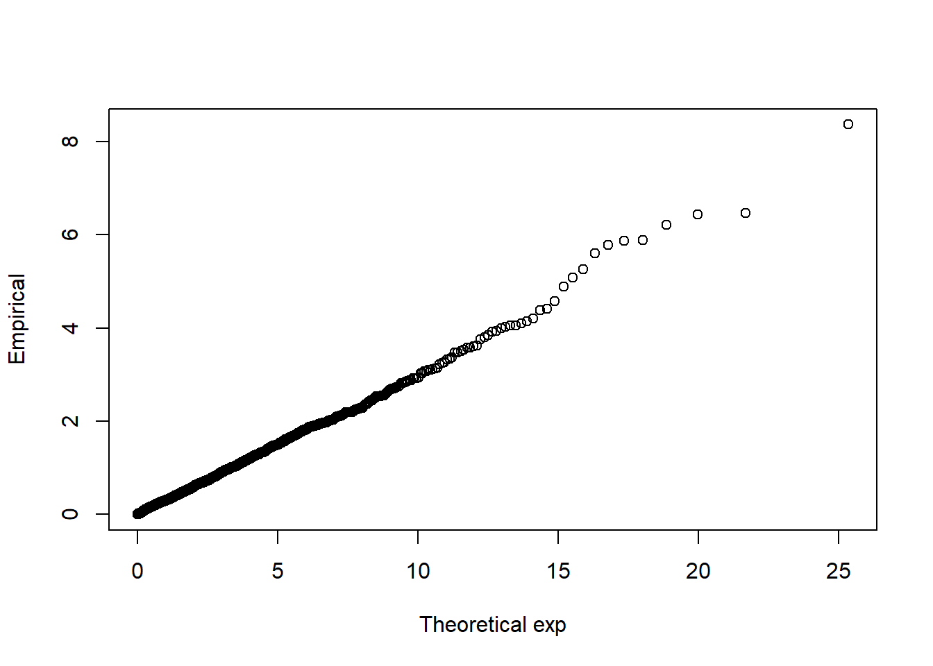 

Further reading

There is a lot of free material online for learning R and good coding practices. Some recommended resources include:

• Introduction to R: http://cran.r-project.org/doc/manuals/R-intro.pdf

• On good coding style: short - http://adv-r.had.co.nz/Style.html

• … detailed: http://cran.r-project.org/web/packages/rockchalk/vignettes/Rstyle.pdf