2.3 Type 1 and type 2 errors
In section 2.2, we explained the logic behind null hypothesis testing: we determine the probability of observing the data we have observed assuming that the null hypothesis is true, and reject the null hypothesis if this probability is lower than 5 percent. We also cautioned, however, that rejecting the null hypothesis or not is a decision that we make. Decisions can be incorrect, and because we don’t know whether, in reality, the null hypothesis is true or not, we cannot evaluate whether a particular decision is correct or incorrect.
There are two types of incorrect decisions that we can make:
- In reality there’s no difference in population means, so \(\mathcal{H_{0}}\) is true, but we decide to reject it. We call this a Type 1 error. A more common term is false positive: we think there is a difference in population means that in reality does not exist.
- In reality there is a difference in population means, so \(\mathcal{H_{0}}\) is false, but we decide not to reject it. We call this a Type 2 error. A more common term is false negative: we think there is no difference in population means but in reality there is.
Depending on the discipline, we are more concerned with one type of error than the other. In justice, guilty people sometimes go free, which is a Type 2 error: the accused was guilty of a crime but the courts let the accused go free. The justice system is more worried, however, about wrongly convicting innocent people, which is a Type 1 error: the accused was not guilty of a crime but the courts convicted the accused. Therefore, the justice system only convicts people when their guilt has been proven beyond reasonable doubt. It tries to maximally avoid committing Type 1 errors. In other disciplines, we may be more concerned with avoiding Type 2 errors than with avoiding Type 1 errors. In medical screening, we really want to avoid missing a cancer that is there (a Type 2 error) as the patient may go about their life without receiving the necessary cancer treatment, and we may be less concerned with wrongly spotting a cancer that isn’t there (a Type 1 error), as this can always be corrected in a second screening. In science, however, we want avoid Type 1 errors more than Type 2 errors, because we don’t to build a science on a foundation of false premises.
Let’s illustrate which situations give rise to Type 1 and Type 2 errors and how we can reduce the risk of making these errors.
2.3.1 Type 1 errors
A Type 1 error occurs when in reality there’s no difference in population means, so \(\mathcal{H_{0}}\) is true, but we observe a difference in sample means that makes us decide there is a difference in population means.
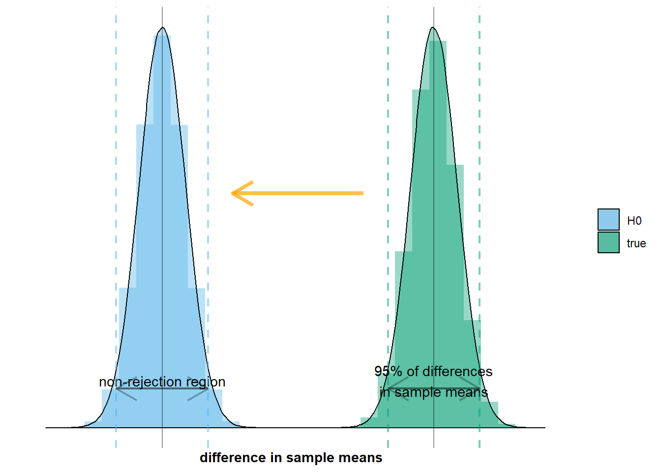
Let’s illustrate the first aspect of this situation: there’s no difference in population means. This means that the true sampling distribution, \(\mathcal{N}(\mu_{men} - \mu_{women}, \frac{\sigma_{men}^2}{n_{men}} + \frac{\sigma_{women}^2}{n_{women}})\), coincides with the null distribution, \(\mathcal{N}(0, \frac{\sigma_{men}^2}{n_{men}} + \frac{\sigma_{women}^2}{n_{women}})\). On the graph below this would mean that the green distribution overlaps with the grey distribution:
resulting in the following graph:
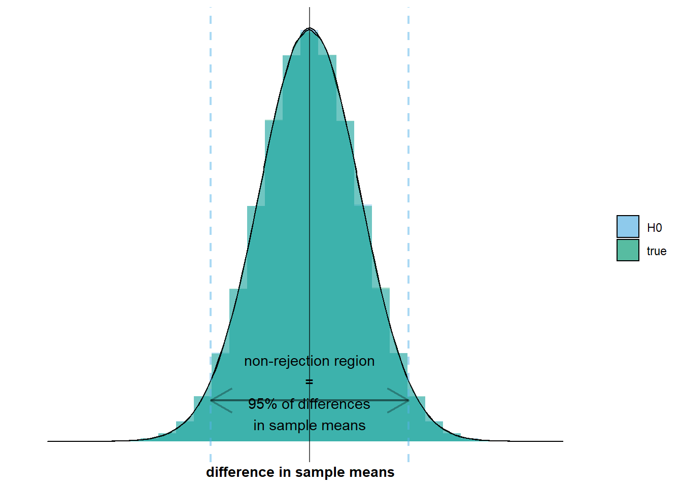
on which we see that the non-rejection region overlaps with the interval where 95% of the differences in sample means will lie. So in 95% of surveys, we will observe a difference in sample means within the non-rejection region. In those cases, we will not reject the null hypothesis, which would be the correct decision. However, and this brings us to the second aspect of the situation, this also means that in 5% of surveys, we will observe a difference in sample means outside the non-rejection region. In those cases, we will reject the null hypothesis, which would be a Type 1 error. I’ve added an example to the graph below:
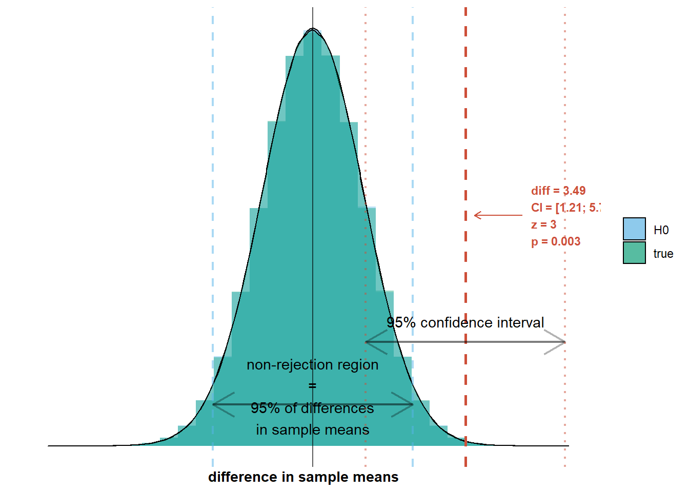
If the null hypothesis is true, we will only observe such a difference in 5% of all surveys, as 95% of surveys will have a difference in sample means within the non-rejection region. So in only 5% of cases will we make a Type 1 error where we reject the null hypothesis even though it is true. We say that the Type 1 error rate, denoted by \(\alpha\), is 5%.
It is important to realize that the Type 1 error rate is fully under our control. We have decided to reject the null hypothesis if we observe a difference in sample means that is at least \(1.96 \times \sqrt{\frac{\sigma_{men}^2}{n_{men}} + \frac{\sigma_{women}^2}{n_{women}}}\) away from zero. If \(\mathcal{H_{0}}\) is true, we observe such a difference in only 5% of surveys, so \(\alpha = 0.05\). There is nothing magical about 5%, however. We could decide that we want a lower Type 1 error rate, say \(\alpha = 0.01\). In that case, we should reject the null hypothesis only if we observe a difference in sample means that is at least \(2.575 \times \sqrt{\frac{\sigma_{men}^2}{n_{men}} + \frac{\sigma_{women}^2}{n_{women}}}\) away from zero. In other words, we widen the non-rejection region. We could also decide to tolerate a higher Type 1 error rate, say \(\alpha = 0.10\). In that case, we should reject the null hypothesis already if we observe a difference in sample means that is \(1.64 \times \sqrt{\frac{\sigma_{men}^2}{n_{men}} + \frac{\sigma_{women}^2}{n_{women}}}\) away from zero. In other words, we shrink the non-rejection region.
In many sciences, \(\alpha = 0.05\) is common. This is why our discussion until now has been based on 95% regions and why the number 1.96 has featured prominently, but it’s important to realize that these numbers derive from a decision to set the Type 1 error rate at 5 percent. Depending on our goals, we can decide to set a different Type 1 error rate.
2.3.2 Type 2 errors
A Type 2 error occurs when in reality there is a difference in population means, so \(\mathcal{H_{0}}\) is false, but we observe a difference in sample means that makes us decide there is no difference in population means.
Let’s illustrate the first aspect of this situation: there is a difference in population means. This means that the true sampling distribution, \(\mathcal{N}(\mu_{men} - \mu_{women}, \frac{\sigma_{men}^2}{n_{men}} + \frac{\sigma_{women}^2}{n_{women}})\), does not fully coincide with the null distribution, \(\mathcal{N}(0, \frac{\sigma_{men}^2}{n_{men}} + \frac{\sigma_{women}^2}{n_{women}})\). On the graph below this would mean that the green distribution does not fully overlap with the grey distribution:
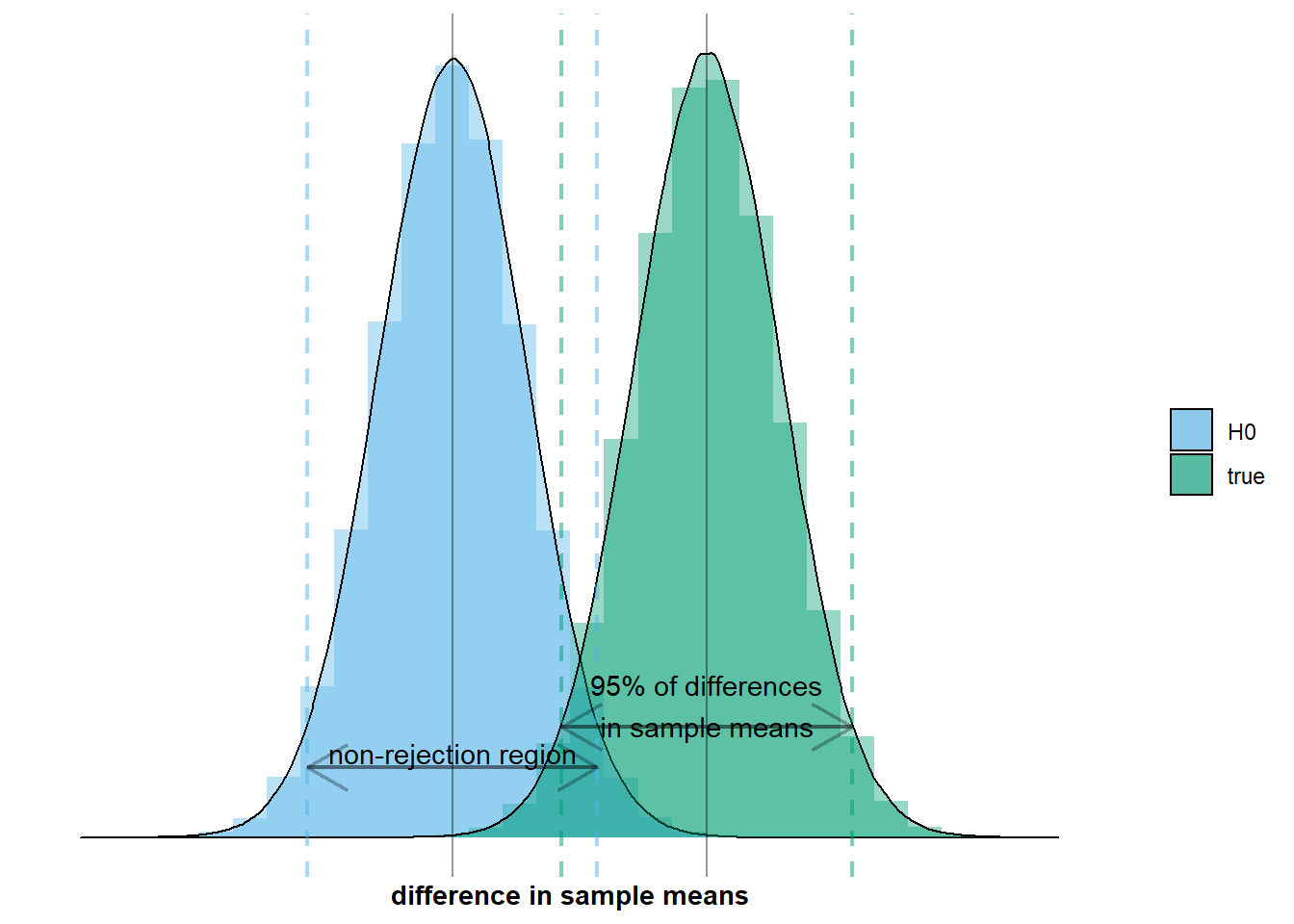
The second aspect of the situation is that we observe a difference in sample means that makes us decide there is no difference in population means. This happens when we observe a difference in sample means inside the non-rejection region. I’ve added an example to the graph below:
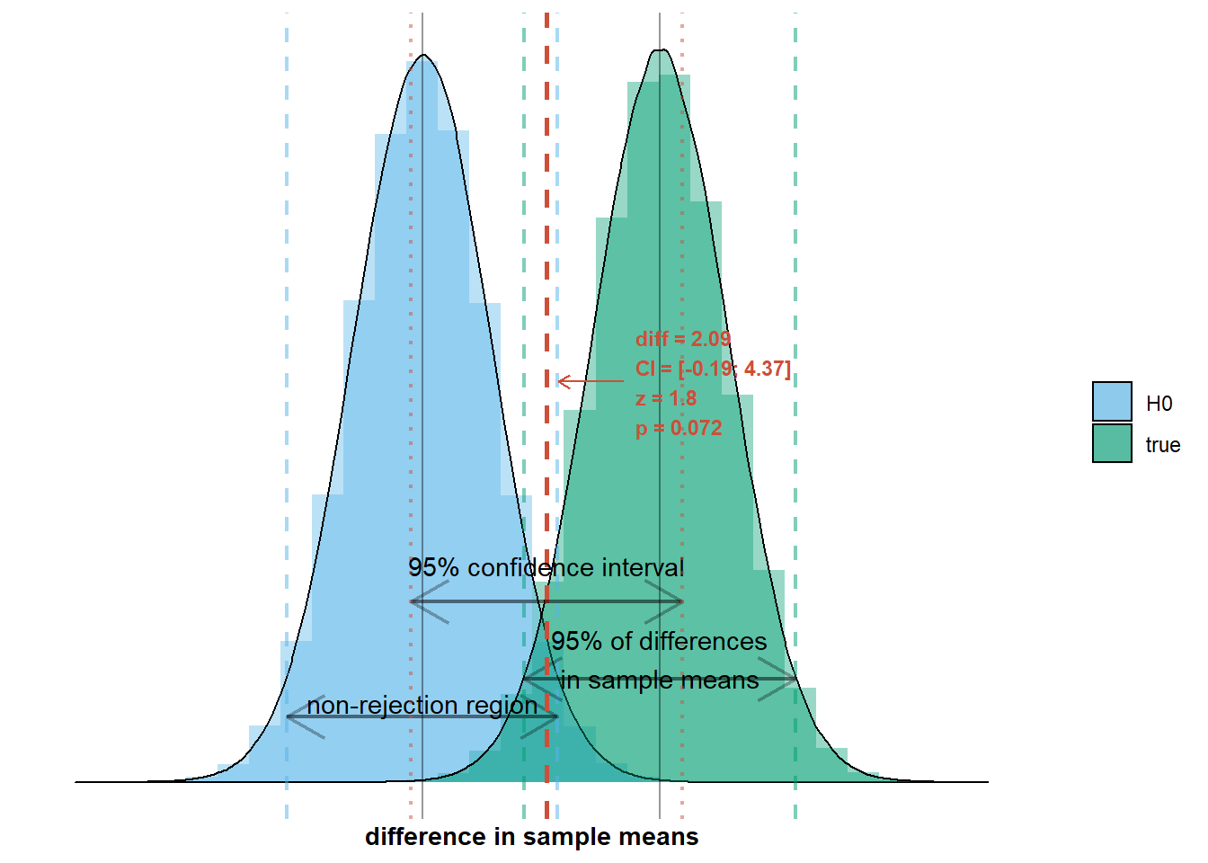
We will observe a difference in sample means within the non-rejection region in a certain percentage of surveys. This percentage is the Type 2 error rate, denoted by \(\beta\). It depends on the width of the non-rejection region and the location and width of the true sampling distribution. The width of the non-rejection region is two times the standard error, \(\sqrt{\frac{\sigma_{men}^2}{n_{men}} + \frac{\sigma_{women}^2}{n_{women}}}\), multiplied by a number that increases with decreasing Type 1 error rate (two times because the interval extends in positive and in negative direction; for \(\alpha = 0.05\), the multiplier is 1.96). So the Type 2 error rate depends on the Type 1 error rate: when the Type 1 error rate is higher (lower), the non-rejection region is narrower (wider) and less (more) differences in sample means will fall within the non-rejection region, so the Type 2 error rate is lower (higher). The number of observations that will fall within the non-rejection region also depends on the mean (location) of the true sampling distribution, \(\mu_{men} - \mu_{women}\), and on the standard deviation (width) of the true sampling distribution, also known as the standard error, \(\sqrt{\frac{\sigma_{men}^2}{n_{men}} + \frac{\sigma_{women}^2}{n_{women}}}\). There will be fewer observations within the non-rejection region when the true sampling distribution has a higher mean and a smaller standard deviation, because most difference in sample means will fall closer to a mean that is farther away from zero and hence the non-rejection region.
Remember that the standard error is under our control. We can lower it by increasing the sample size. Hence, the Type 2 error rate will be lower when sample sizes increase. So with increasing n, we will increasingly avoid the mistake of incorrectly not rejecting \(\mathcal{H_{0}}\), hence we will increasingly often correctly reject the \(\mathcal{H_{0}}\). The percentage of surveys in which we will correctly reject the null hypothesis, denoted by \(1 - \beta\), is also called the statistical power of our test.
Refer to app