2.1 Population versus samples
2.1.1 Population distribution of height among men & women
In the population of men, height is normally distributed with a mean of \(\mu_{men}= 176\) and a standard deviation of \(\sigma_{men}= 7.1\) (\(\sigma\) is the Greek letter s and represents the population standard deviation).

Because height is normally distributed, we can apply the empirical rule. This rule tells us that 95% of men are within 1.96 standard deviations from the mean. The graph confirms this: 95% of men are between \(\mu_{men}\pm 1.96 \times\sigma_{men}= 176 \pm 1.96 \times 7.1 = [162.1; 189.9]\) centimeters tall. In other words, if we pick a random man from the population, there’s a 95% probability that he’s between 162.1 and 189.9 centimeters tall.
Among women, height is normally distributed with a mean of \(\mu_{women}= 162.5\) and a standard deviation of \(\sigma_{women}= 7.1\).

According to the empirical rule, 95% of women are within 1.96 standard deviations from the mean. The graph confirms this: 95% of women are between \(\mu_{women}\pm 1.96 \times\sigma_{women}= 162.5 \pm 1.96 \times 7.1 = [148.6; 176.4]\) centimeters tall. In other words, if we pick a random woman from the population, there’s a 95% probability that she’s between 148.6 and 176.4 centimeters tall.
Let’s put these two plots together:
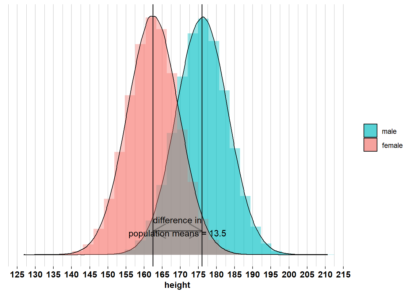
We see that the difference in population means is \(\mu_{men} - \mu_{women}= 13.5\), so the average man is 13.5 centimeters taller than the average woman. This means that if we pick a random man and a random woman from the population, the most likely difference in height is 13.5 centimeters. We also see, however, that there is a lot of overlap between men and women. A random person of 169.25 centimeters tall is equally likely to be a man or a woman. So the fact that the average is higher for men than for women does not necessarily mean that most men are taller than most women. The overlap of the distributions is also determined by the variation in height among men and among women. If this variation is small, then there will be little overlap, which means that most men are taller than most women. If this variation is large, then there will be quite some overlap, which means that only the tallest men are taller than most women and only the shortest women are shorter than most men.
Let’s now turn our attention to the data we observed in our survey.
2.1.2 The actual survey and resulting samples
The survey resulted in a sample of \(\mathcal{n}_{men}= 74\) men and a sample of \(\mathcal{n}_{women}= 75\) women. Let’s visualize their heights in a histogram:
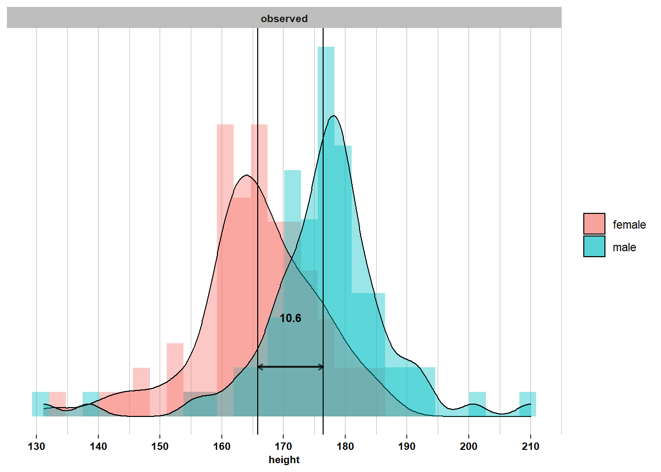
We see that the distribution of height is roughly normal for the sample of men and for the sample of women. The average man in the sample is \(\bar{x}_{men}= 176.4\) centimeters tall, which is very similar to the population mean for men (\(\mu_{men}= 176\)). The average woman in the sample is \(\bar{x}_{women}= 165.8\) centimeters tall, which is quite a bit taller than the population mean for women (\(\mu_{women}= 162.5\)).
If we calculate the 2.5th and 97.5th percentiles, we see that 95% of men in the sample are between 152.3 and 194.6 centimeters tall, which corresponds to the 95% interval in the population ([162.1; 189.9]). For women, however, the 95% interval in the sample ([142.6; 183.3]) is higher than that of the population ([148.6; 176.4]).
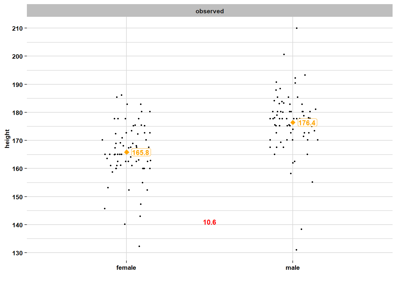
So overall, the samples of men and women look roughly like the populations, but they’re not perfect mirror images of the populations. Below is the same information, but now in a scatterplot:
2.1.3 Other possible surveys and resulting samples
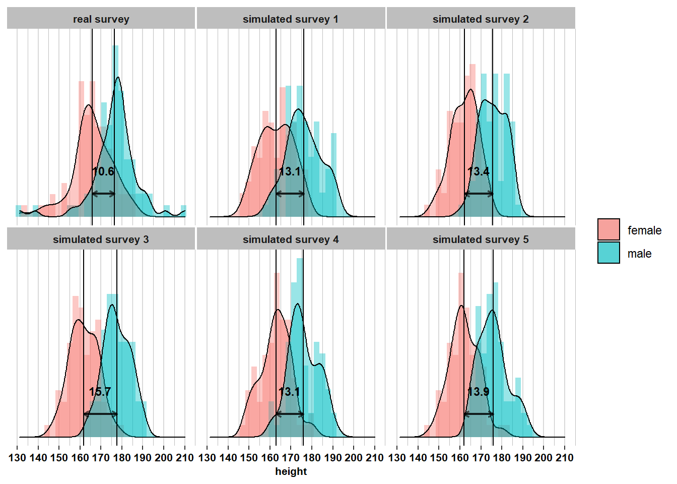
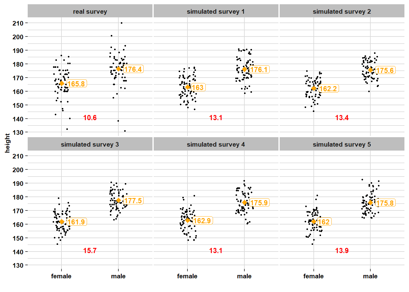
Samples do not perfectly mirror populations, because the process of sampling introduces randomness. In the samples we have drawn, we noticed, for example, that the 75 women were relatively tall compared to the population of women. It’s important to understand, however, that the samples we have observed could have been different. If other US citizens had filled in the survey, then we would have observed different sample means for men and for women. This is where the randomness comes in: the people who fill in the survey are not the same people from survey to survey. Therefore, if we would re-run the survey many times, we would observe different means in each of the resulting samples. Let’s visualize this. I’ve simulated another five surveys with \(\mathcal{n}_{men}= 74\) and \(\mathcal{n}_{women}= 75\):
This is the same information, but now in a scatterplot:
Again, the same information, but now in a table:
## # A tibble: 12 x 7
## # Groups:   sample [6]
##    gender sample                 n  mean    sd  q025  q975
##    <chr>  <fct>              <dbl> <dbl> <dbl> <dbl> <dbl>
##  1 female real survey           75  166.  10    143.  183.
##  2 female simulated survey 1    72  163    7.9  150.  177.
##  3 female simulated survey 2    72  162.   6.5  149.  173.
##  4 female simulated survey 3    72  162.   6.9  150.  175.
##  5 female simulated survey 4    72  163.   7.3  148.  178.
##  6 female simulated survey 5    72  162    6.9  150.  174.
##  7 male   real survey           74  176.  11.2  152.  195.
##  8 male   simulated survey 1    71  176.   8.2  161.  190.
##  9 male   simulated survey 2    71  176.   6.3  164   185.
## 10 male   simulated survey 3    71  178.   6.5  165.  190.
## 11 male   simulated survey 4    71  176.   7.1  162.  188.
## 12 male   simulated survey 5    71  176.   7.1  165.  191.
On the graphs and in the table, we see that, for each sample, the sample means are quite close to the population means. We also see that within each sample, the distributions look roughly normal, with 95% of men roughly between 162 and 190 centimeters, and 95% of women roughly between 148 and 177 centimeters. These intervals correspond quite closely to the equivalent intervals at the population level (where 95% of men are in [162.1; 189.9] and 95% of women are in [148.6; 176.4]). Overall, each sample differs from the next sample, but each sample also looks roughly like the population.
However, let’s now look at how much the means differ from sample to sample. We see that in these 6 surveys, the sample means among men vary from 175.6 to 177.5 (range = 1.9) and the sample means among women vary from 161.9 to 165.8 (range = 3.9). This between-sample variation in means is much lower than the within-sample variation between individuals. This is because it’s hard for a sample mean to deviate strongly from the corresponding population mean. To obtain a sample mean that deviates strongly from the population mean, you would have to sample mostly tall (or short) people and somehow avoid short (or tall) people. This could happen in small samples, but it’s unlikely to happen in larger samples: it’s relatively easy to run into three people who are all relatively tall (or short), but much harder to run into thirty people who are all relatively tall (or short). The larger the sample, the more it will look like the population, where you have a mixture of tall and short people and everyone in between. Therefore, the sample means will resemble the population means and they will differ between samples to a much lesser extent than the individual people will differ within samples.
2.1.4 Distribution of sample means
Let’s formalize the above intuition. If \(X\) is a normally distributed random variable with population mean \(\mu_{X}\) and population variance \(\sigma_{X}^2\), then the mean of a sample of \(n\) independent observations of \(X\) is also a normally distributed random variable, \(\bar{X}\), with mean \(\mu_{\bar{X}} = \mu_{X}\), but variance \(\sigma_{\bar{X}}^2 = \frac{\sigma_{X}^2}{n}\). Formally, if \(X \sim \mathcal{N}(\mu_{X}, \sigma_{X}^2)\), then \(\bar{X}\sim \mathcal{N}(\mu_{X}, \frac{\sigma_{X}^2}{n})\). Note that we consider \(\bar{X}\) as a random variable: the value of \(\bar{X}\) differs from sample to sample because each sample will have different observations of which we calculate the mean. The distribution of \(\bar{X}\) describes how the sample means differ from sample to sample. It is also called a sampling distribution (this is the term that we use for the distribution of a statistic).
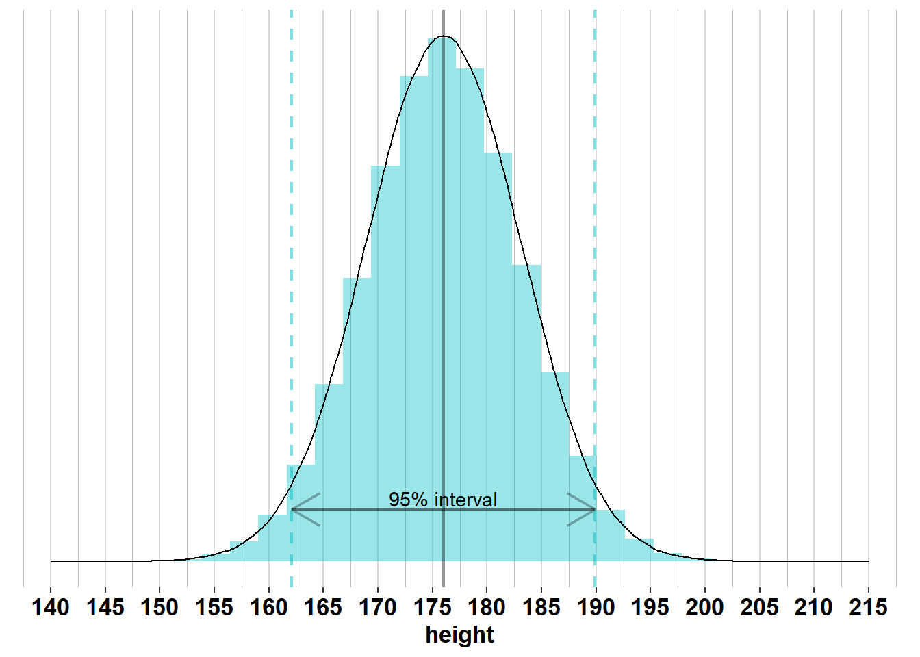
Comparing the distributions of \(X\) and \(\bar{X}\) tells us that height will vary much more between individuals in a sample than average height will vary between samples, because \(\sigma_{X}^2 > \frac{\sigma_{X}^2}{n}\). In the example of height in the US, we know that the height of men is normally distributed with \(\mu_{men}= 176\) and \(\sigma_{men}= 7.1\). Therefore, 95% of men will have a height between \(\mu_{men}\pm 1.96 \times\sigma_{men}= [162.1; 189.9]\), as you can see in the following graph:
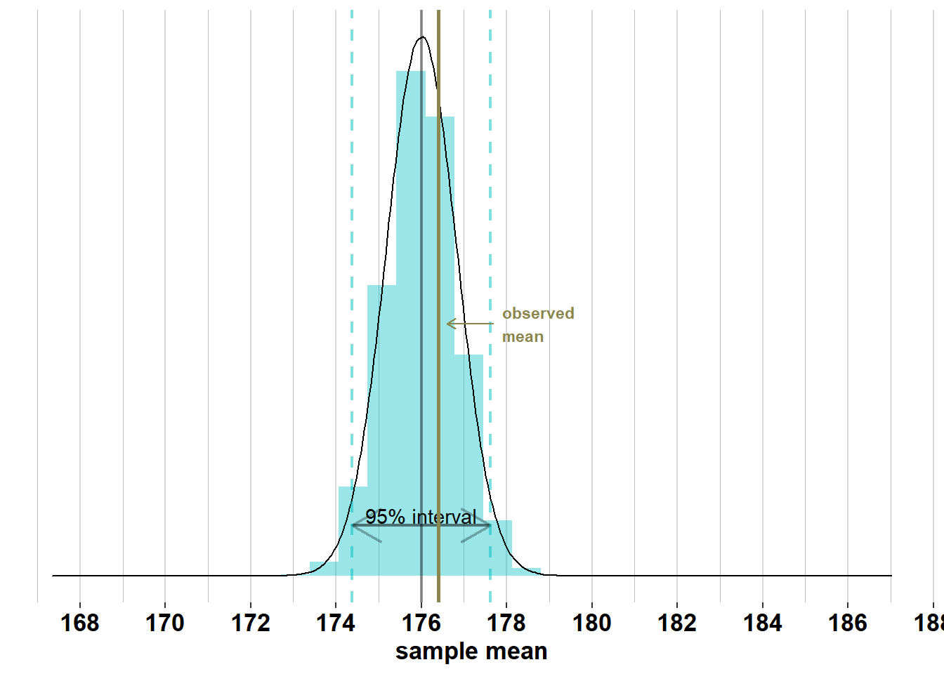
However, in 95% of samples of size \(\mathcal{n}_{men}= 74\), the mean will lie between \(\mu_{men}\pm 1.96 \times\frac{\sigma_{men}}{\sqrt{n}} = [174.4; 177.6]\):
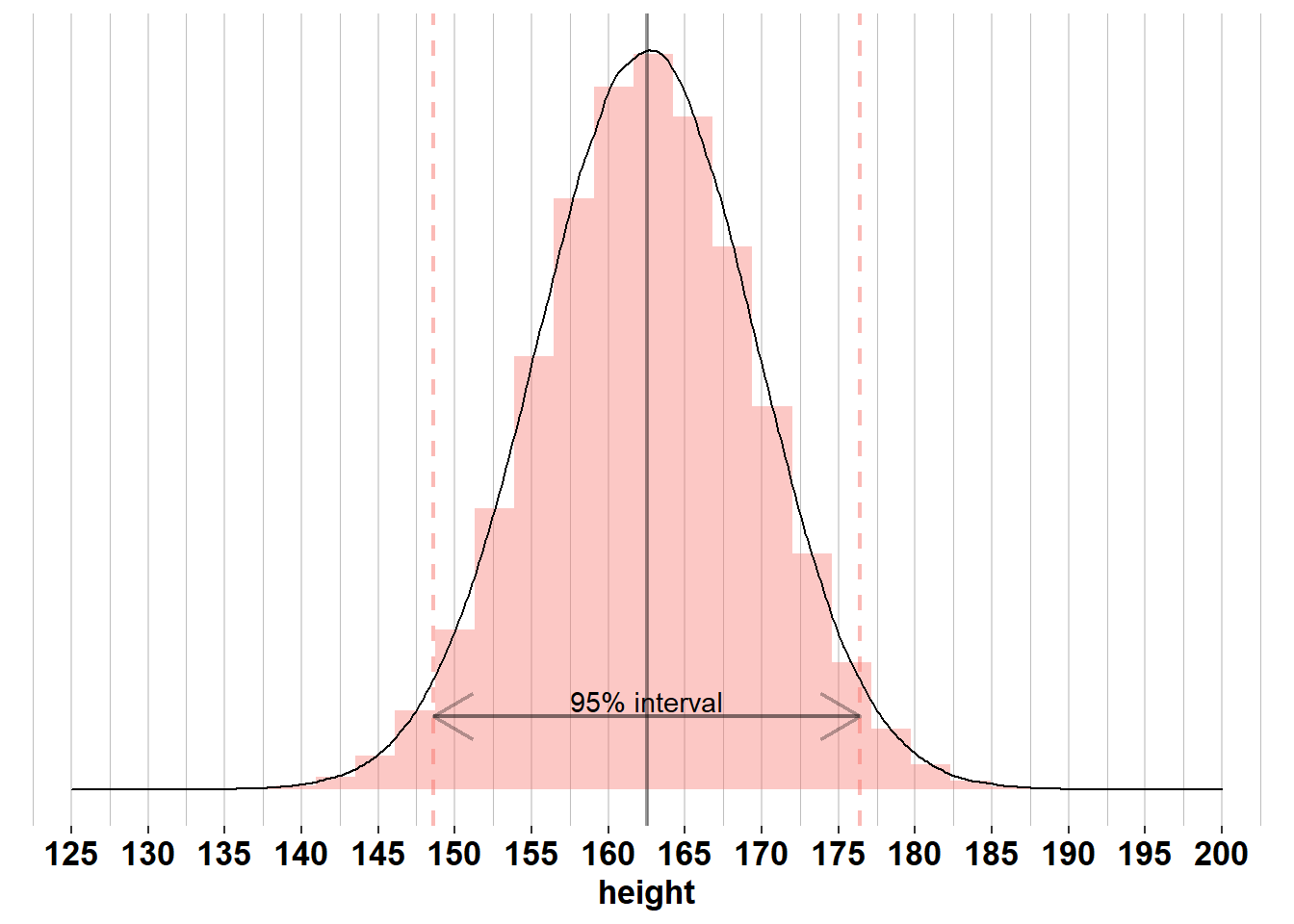
Same reasoning for women. The height of women is normally distributed with \(\mu_{women}= 162.5\) and \(\sigma_{women}= 7.1\), so 95% of women will have a height between \(\mu_{women}\pm 1.96 \times\sigma_{women}= [148.6; 176.4]\):
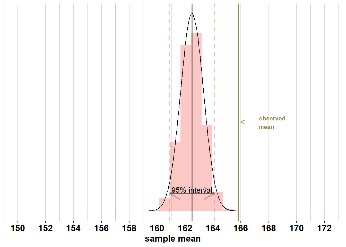
But in 95% of samples of size \(\mathcal{n}_{women}= 75\), the mean will lie between \(\mu_{women}\pm 1.96 \times\frac{\sigma_{women}}{\sqrt{n}} = [160.9; 164.1]\):
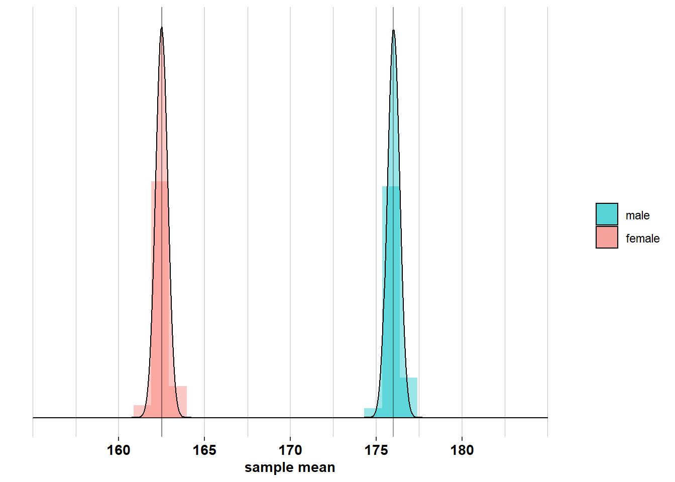
From the distribution of \(\bar{X}\sim \mathcal{N}(\mu_{X}, \frac{\sigma_{X}^2}{n})\), we learn that the larger the sample, the less variation there will be between sample means, because \(\frac{\sigma_{X}^2}{n}\) decreases as \(n\) increases. To understand this, imagine two scenarios. In scenario 1, you carry out 100 surveys, each with \(\mathcal{n}_{men}= 10\) men and \(\mathcal{n}_{women}= 10\) women. In scenario 2, you also carry out 100 surveys, but now each survey samples \(\mathcal{n}_{men}= 20\) men and \(\mathcal{n}_{women}= 20\) women. If you would calculate the 100 \(\bar{x}_{men}\)’s and \(\bar{x}_{women}\)’s in both scenarios, you will notice that there is less variation among the sample means in scenario 2 (where the standard deviations are \(\frac{\sigma_{men}}{20} = \frac{\sigma_{women}}{20}\)):
than in scenario 1 (where the standard deviations are \(\frac{\sigma_{men}}{10} = \frac{\sigma_{women}}{10}\)):
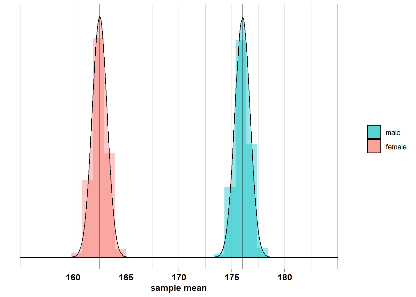
This is because in scenario 2, the sample sizes are larger and the means will lie closer, on average, to the population means, than in scenario 1. In general, as \(n\) increases, the sample means \(\bar{x}\) will lie closer to the mean of their distribution \(\mu_{\bar{X}} = \mu_{X}\).
2.1.5 Distribution of the difference in sample means
In the above, we looked at how the sample means vary from survey to survey. We can also look at how the difference in sample means varies from survey to survey. You can see this on the histograms or scatterplots from section 2.1.3 or in this table below:
## # A tibble: 6 x 4
## # Groups:   sample [6]
##   sample             female  male difference
##   <fct>               <dbl> <dbl>      <dbl>
## 1 real survey          166.  176.       10.6
## 2 simulated survey 1   163   176.       13.1
## 3 simulated survey 2   162.  176.       13.4
## 4 simulated survey 3   162.  178.       15.6
## 5 simulated survey 4   163.  176.       13
## 6 simulated survey 5   162   176.       13.8
Across these 6 surveys, these differences range from 10.6 to 15.6 and are quite close to the difference in population means \(\mu_{men} - \mu_{women}= 13.5\). Again, we can mathematically derive the distribution of the difference in sample means:
- If \(X_{men} \sim \mathcal{N}(\mu_{men}, \sigma_{men}^2)\) and \(X_{women} \sim \mathcal{N}(\mu_{women}, \sigma_{women}^2)\),
- then \(\bar{X}_{men}\sim \mathcal{N}(\mu_{men}, \frac{\sigma_{men}^2}{n_{men}})\) and \(\bar{X}_{women}\sim \mathcal{N}(\mu_{women}, \frac{\sigma_{women}^2}{n_{women}})\),
- and \(\bar{X}_{men}- \bar{X}_{women}\sim \mathcal{N}(\mu_{men} - \mu_{women}, \frac{\sigma_{men}^2}{n_{men}} + \frac{\sigma_{women}^2}{n_{women}})\).
We call this the sampling distribution of the difference in sample means (as explained in section 2.1.4, \(\bar{X}_{men}- \bar{X}_{women}\) is a random variable). If we apply the empirical rule to this distribution, we know that in 95% of surveys, the difference in sample means will lie between \(\mu_{men} - \mu_{women}\pm 1.96 \times\sqrt{\frac{\sigma_{men}^2}{n_{men}} + \frac{\sigma_{women}^2}{n_{women}}}\). In this case, this means that 95% of surveys will have a difference in sample means between \(13.5 \pm 1.96 \times 1.16 = [11.2; 15.8]\):
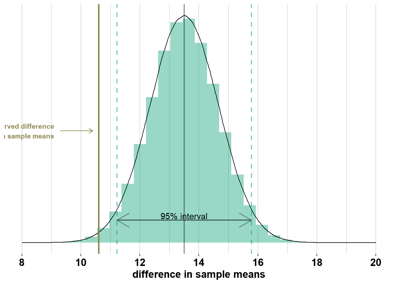
The difference in sample means that we have observed (\(\bar{x}_{men}- \bar{x}_{women}\) = 10.6) is lower than 95% of these differences.
2.1.6 The Z-transformation of the difference in sample means
The difference in sample means is an important statistic. We know that it follows a normal distribution: \(\bar{X}_{men}- \bar{X}_{women}\sim \mathcal{N}(\mu_{men} - \mu_{women}, \frac{\sigma_{men}^2}{n_{men}} + \frac{\sigma_{women}^2}{n_{women}})\). The standard deviation of the distribution of the difference in sample means \(\sqrt{\frac{\sigma_{men}^2}{n_{men}} + \frac{\sigma_{women}^2}{n_{women}}}\) is also called the standard error.
However, let’s linearly transform the difference in sample means into a new statistic that we call \(Z\) and that is equal to dividing the difference in sample means by the standard error:
\(Z = \frac{\bar{x}_{men}- \bar{x}_{women}}{\sqrt{\frac{\sigma_{men}^2}{n_{men}} + \frac{\sigma_{women}^2}{n_{women}}}}\).
In our example, this would mean taking the difference in sample means and dividing it by \(\sqrt{\frac{7.1²}{74} + \frac{7.1²}{75}} = 1.16\). The table below contains the resulting \(Z\)-scores for each survey (one real and 6 simulated):
## # A tibble: 6 x 5
## # Groups:   sample [6]
##   sample             female  male difference     Z
##   <fct>               <dbl> <dbl>      <dbl> <dbl>
## 1 real survey          166.  176.       10.6   9.1
## 2 simulated survey 1   163   176.       13.1  11.3
## 3 simulated survey 2   162.  176.       13.4  11.5
## 4 simulated survey 3   162.  178.       15.6  13.4
## 5 simulated survey 4   163.  176.       13    11.2
## 6 simulated survey 5   162   176.       13.8  11.9
This is an interesting transformation because \(Z\) is distributed as \(Z \sim \mathcal{N}(\frac{\mu_{men} - \mu_{women}}{\sqrt{\frac{\sigma_{men}^2}{n_{men}} + \frac{\sigma_{women}^2}{n_{women}}}}, 1)\). This will come in useful later on.
In this example, \(Z \sim \mathcal{N}(\frac{13.5}{1.16}, 1)\) or \(Z \sim \mathcal{N}(11.6, 1)\). Applying the empirical rule, we know that in 95% of surveys, we will observe a \(Z\)-score within \(11.6 \pm 1.96 \times 1 = [9.64 ; 13.56]\).