2.2 Null hypothesis testing
In the previous section, we have discussed the population distributions of height among men and women in the US, and the resulting samples we are bound to observe. However, when faced with a real data analysis problem, we don’t know the population distributions of the variables involved. If we did, we would not have to collect data to figure out whether \(\mu_{men} - \mu_{women}> 0\), because we would just know this information already. Instead, we need to make an informed guess about whether \(\mu_{men} - \mu_{women}> 0\), based on the difference in sample means, \(\bar{x}_{men}- \bar{x}_{women}\). The question is: given the observed difference in sample means, how likely is it that the difference in population means is positive? However, in (frequentist) statistics, we turn this question around: If the population difference in means were zero, what would be the likelihood of observing the difference in sample means that we have observed? If this likelihood turns out to be really low, then we reject the assumption that the population difference in means is zero.
The logic of null hypothesis testing is as follows:
- Step 1: We assume that \(\mu_{men} - \mu_{women}= 0\). We call this assumption the null hypothesis or \(\mathcal{H_{0}}\).
- Step 2: If the null hypothesis is true, then the difference in sample means \(\bar{X}_{men}- \bar{X}_{women}\) follows a normal distribution \(\mathcal{N}(\mu_{men} - \mu_{women}, \frac{\sigma_{men}^2}{n_{men}} + \frac{\sigma_{women}^2}{n_{women}})\). Under \(\mathcal{H_{0}}: \mu_{men} - \mu_{women}= 0\), this becomes \(\mathcal{N}(0, \frac{\sigma_{men}^2}{n_{men}} + \frac{\sigma_{women}^2}{n_{women}})\). If we apply the empirical rule, we know that 95% of surveys will have a difference in sample means between \(\mu_{men} - \mu_{women}\pm 1.96 \times\sqrt{\frac{\sigma_{men}^2}{n_{men}} + \frac{\sigma_{women}^2}{n_{women}}}\). Under \(\mathcal{H_{0}}: \mu_{men} - \mu_{women}= 0\), this becomes \(0 \pm 1.96 \times\sqrt{\frac{\sigma_{men}^2}{n_{men}} + \frac{\sigma_{women}^2}{n_{women}}}\). We call this interval the non-rejection region.
- Step 3: We compare the observed difference in sample means, \(\bar{x}_{men} - \bar{x}_{women}\), with the non-rejection region. Differences in sample means that fall within the non-rejection region are differences you expect to observe in 95% of surveys when \(\mathcal{H_{0}}\) is true, so they are not unusual for \(\mathcal{H_{0}}\). These differences in sample means give no reason to doubt that \(\mathcal{H_{0}}\) is true, so we do not reject \(\mathcal{H_{0}}\). Differences in sample means that fall outside the non-rejection region are differences you expect to observe in only 5% of surveys when \(\mathcal{H_{0}}\) is true, so they are unusual for \(\mathcal{H_{0}}\). These differences in sample means do give reason to doubt that \(\mathcal{H_{0}}\) is true, so we reject \(\mathcal{H_{0}}\).
Note that this becomes easier if we make use of the \(Z\)-transformation:
- Step 2: we know that if \(\bar{X}_{men}- \bar{X}_{women}\sim \mathcal{N}(\mu_{men} - \mu_{women}, \frac{\sigma_{men}^2}{n_{men}} + \frac{\sigma_{women}^2}{n_{women}})\), then \(Z \sim \mathcal{N}(\frac{\mu_{men} - \mu_{women}}{\sqrt{\frac{\sigma_{men}^2}{n_{men}} + \frac{\sigma_{women}^2}{n_{women}}}}, 1)\). Under \(\mathcal{H_{0}}: \mu_{men} - \mu_{women}= 0\), \(Z \sim \mathcal{N}(0, 1)\). We call this normal distribution with mean zero and variance one, the standard normal distribution. If we apply the empirical rule, we know that 95% of surveys will have a difference in sample means between \(0 \pm 1.96 \times 1\), which is the non-rejection region. So, regardless of the mean and standard deviation of \(\bar{X}_{men}- \bar{X}_{women}\), \(Z\) follows a standard normal distribution under \(\mathcal{H_{0}}\), and the non-rejection region is \([-1.96; 1.96]\). Therefore, step 2 requires no calculation.
- Step 3: we only need to \(Z\)-transform the difference in sample means and compare it to the non-rejection region [-1.96; 1.96]. If \(z = \frac{\bar{x}_{men} - \bar{x}_{women}}{\sqrt{\frac{\sigma_{men}^2}{n_{men}} + \frac{\sigma_{women}^2}{n_{women}}}}\) is within [-1.96; 1.96], we don’t reject \(\mathcal{H_{0}}\); if it’s outside [-1.96; 1.96], we reject \(\mathcal{H_{0}}\).
In the following, we will demonstrate this line of reasoning with the example of height among men and women in the United States. Keep in mind, however, that rejecting or not rejecting \(\mathcal{H_{0}}\) is a decision we make based on the data in our sample. These decisions may of course be wrong. The null hypothesis could be true in reality, but we may observe a difference in sample means that leads us to reject it, or the null hypothesis could be false in reality, but we may observe a difference in sample means that leads us to not reject it. Both types of error will be discussed in more detail in section 2.3.
2.2.1 Rejecting the null hypothesis versus not
We want to test whether \(\mathcal{H_{0}}: \mu_{men} - \mu_{women}= 0\) is true, so we compare the observed \(\bar{x}_{men}- \bar{x}_{women}\) with the distribution of \(\bar{X}_{men}- \bar{X}_{women}\) under \(\mathcal{H_{0}}\). Under \(\mathcal{H_{0}}\), \(\bar{X}_{men}- \bar{X}_{women}\sim \mathcal{N}(0, \frac{\sigma_{men}^2}{n_{men}} + \frac{\sigma_{women}^2}{n_{women}})\). This distribution and the observed \(\bar{x}_{men}- \bar{x}_{women}= 10.6\) are shown on the graph below:
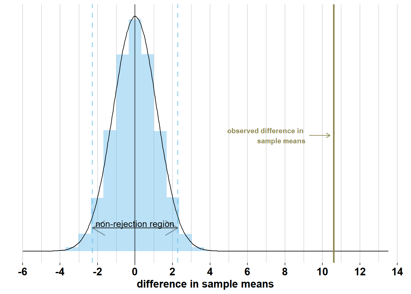
We see on this graph that, if \(\mathcal{H_{0}}\) were true, 95% of surveys would have a difference in sample means within \(0 \pm 1.96 \times\sqrt{\frac{\sigma_{men}^2}{n_{men}} + \frac{\sigma_{women}^2}{n_{women}}}= 0 \pm 1.96 \times\sqrt{\frac{7.1^2}{74} + \frac{7.1^2}{75}} = [-2.28; 2.28]\). We call this the non-rejection region. If the difference in sample means falls within this region, then we will not reject the null hypothesis. However, the difference in sample means that we observed, \(\bar{x}_{men}- \bar{x}_{women}\) = 10.6, is far outside this interval, hence we reject \(\mathcal{H_{0}}\).
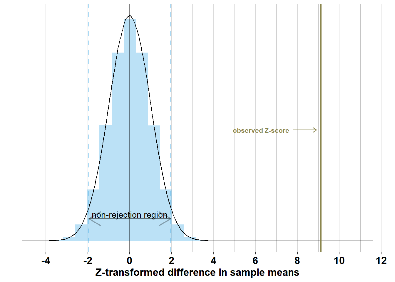
To make this process easier, we can transform \(\bar{x}_{men}- \bar{x}_{women}\) into a \(z\)-score by dividing it by the standard error: \(\frac{\bar{x}_{men}- \bar{x}_{women}}{\sqrt{\frac{\sigma_{men}^2}{n_{men}} + \frac{\sigma_{women}^2}{n_{women}}}} = \frac{176.4-165.8}{1.16} = 9.11\). This is far outside the non-rejection \([-1.96; +1.96]\), hence we reject \(\mathcal{H_{0}}\). As the \(Z\)-transformation is a linear transformation of the differences in sample means, the graph below is the same as the graph above, but with a re-scaled X-axis:
In this case, we know that rejecting \(\mathcal{H_{0}}\) is the correct decision, but remember that we never know the true distributions of the variables of interest, and hence we never know whether a particular decision is correct or not.
2.2.2 p-values
Testing whether two population means are equal is fairly easy: we calculate the \(z\)-score for the observed difference in sample means and reject \(\mathcal{H_{0}}\) when the \(z\)-score is outside the non-rejection region [-1.96; 1.96]. This comes down to rejecting \(\mathcal{H_{0}}\) when we observe a difference in sample means that we should observe, assuming \(\mathcal{H_{0}}\) is true, in only 5% of surveys.
An equivalent method is to calculate the probability, assuming \(\mathcal{H_{0}}\) is true, of observing a difference in sample means as extreme or extremer than the one we have observed. We call this probability the p-value. If the p-value is lower than 5%, we reject \(\mathcal{H_{0}}\). In practice, we will not calculate p-values by hand, but they will feature in the output of statistical tests in every software package.
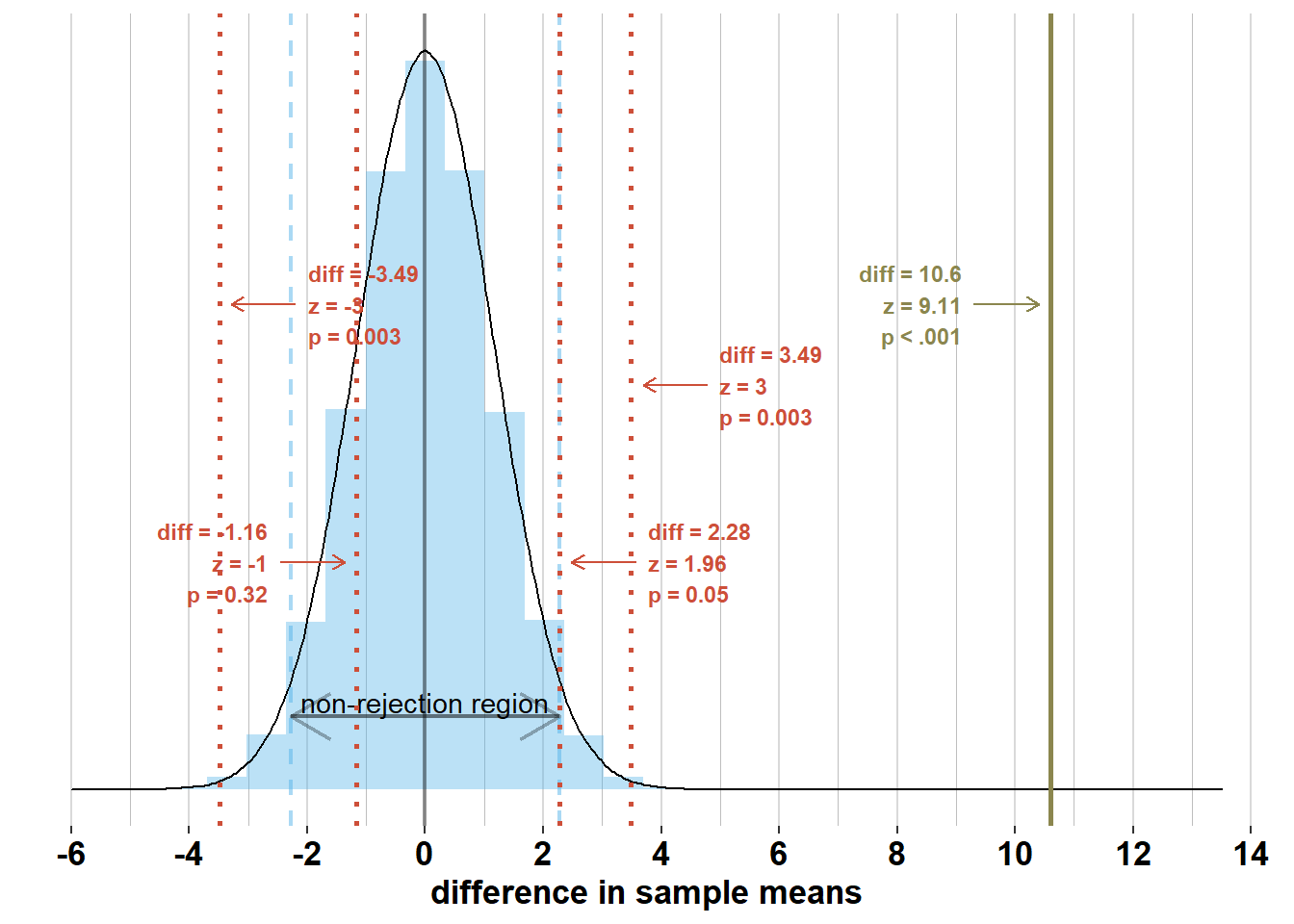
Check out the graph below where I’ve added several potential differences in sample means (“diff”) and the accompanying z-scores and p-values. This graph shows that differences in sample means within the non-rejection region, will have \(z\)-scores within [-1.96; 1.96] and p-values > .05; differences in sample means outside the non-rejection region, will have \(z\)-scores outside [-1.96; 1.96] and p-values < .05.
2.2.3 Confidence intervals
Often, we’re not interested only in rejecting \(\mathcal{H_{0}}\) or not. We may also want to estimate the magnitude of the difference in population means, \(\mu_{men} - \mu_{women}\). To estimate \(\mu_{men} - \mu_{women}\), we use the difference in sample means, \(\bar{x}_{men} - \bar{x}_{women}\). Estimates come with uncertainty, however. The uncertainty in this case is \(\pm 1.96 \times\sqrt{\frac{\sigma_{men}^2}{n_{men}} + \frac{\sigma_{women}^2}{n_{women}}}\) around \(\bar{x}_{men} - \bar{x}_{women}\). We call this interval the 95% confidence interval. The informal interpretation of this confidence interval is that we are 95% confident that the interval contains the difference in population means \(\mu_{men} - \mu_{women}\).
Below, I’ve added the confidence interval to the difference in sample means that we observed in our survey:
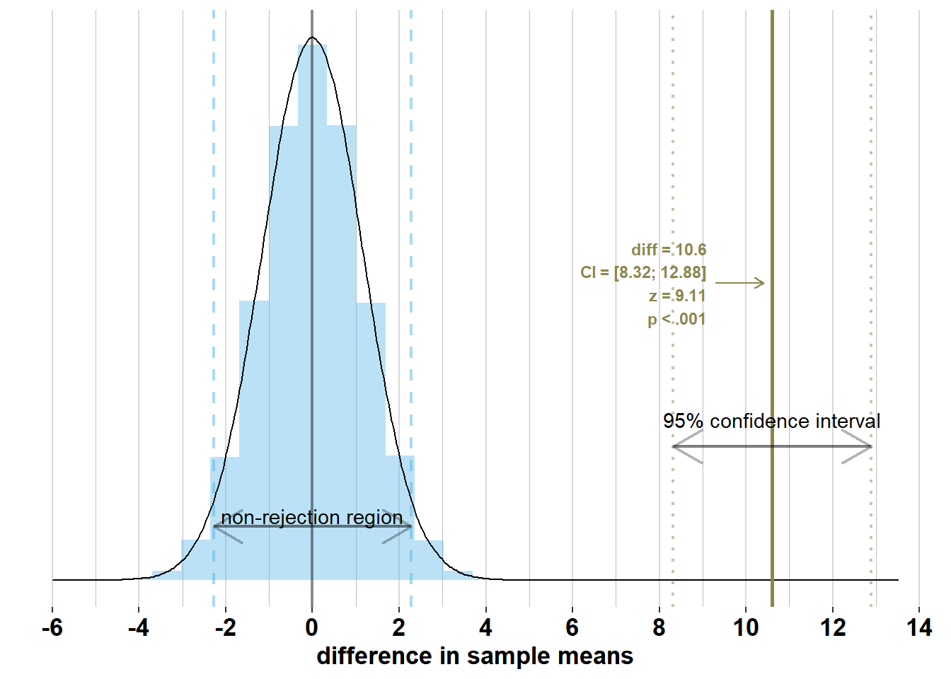
However, this confidence interval, \(\bar{x}_{men} - \bar{x}_{women}\pm 1.96 \times\sqrt{\frac{\sigma_{men}^2}{n_{men}} + \frac{\sigma_{women}^2}{n_{women}}}= 176.4 - 165.8 \pm 1.96 \times\sqrt{\frac{7.1^2}{74} + \frac{7.1^2}{75}} = [8.32; 12.88]\), does not contain the difference in population means, \(\mu_{men} - \mu_{women}= 13.5\). This is because the difference in sample means is outside the interval around the difference in population means where 95% of the differences in sample means will lie, if you would actually do the survey many times (we get this interval by applying the empirical rule to the sampling distribution: \(\mu_{men}- \mu_{women}\pm 1.96 \times\sqrt{\frac{\sigma_{men}^2}{n_{men}} + \frac{\sigma_{women}^2}{n_{women}}}\)). To illustrate this, let’s add the true sampling distribution of the differences in sample means to the graph:
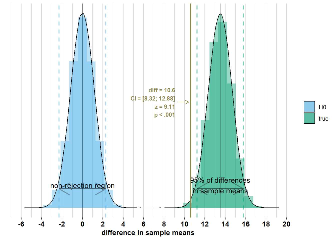
Notice that the observed difference in sample means is outside the interval where 95% of the differences in sample means will lie. Because the observed difference in sample means is more than \(1.96 \times \sqrt{\frac{\sigma_{men}^2}{n_{men}} + \frac{\sigma_{women}^2}{n_{women}}}\) away from the difference in population means, the confidence intervals of width \(\pm 1.96 \times\sqrt{\frac{\sigma_{men}^2}{n_{men}} + \frac{\sigma_{women}^2}{n_{women}}}\) around this difference will not include the difference in population means. Let’s, however, inspect some differences in sample means inside the 95% interval where most differences in sample means will lie (I made a different graph for every observed difference to avoid visual clutter):
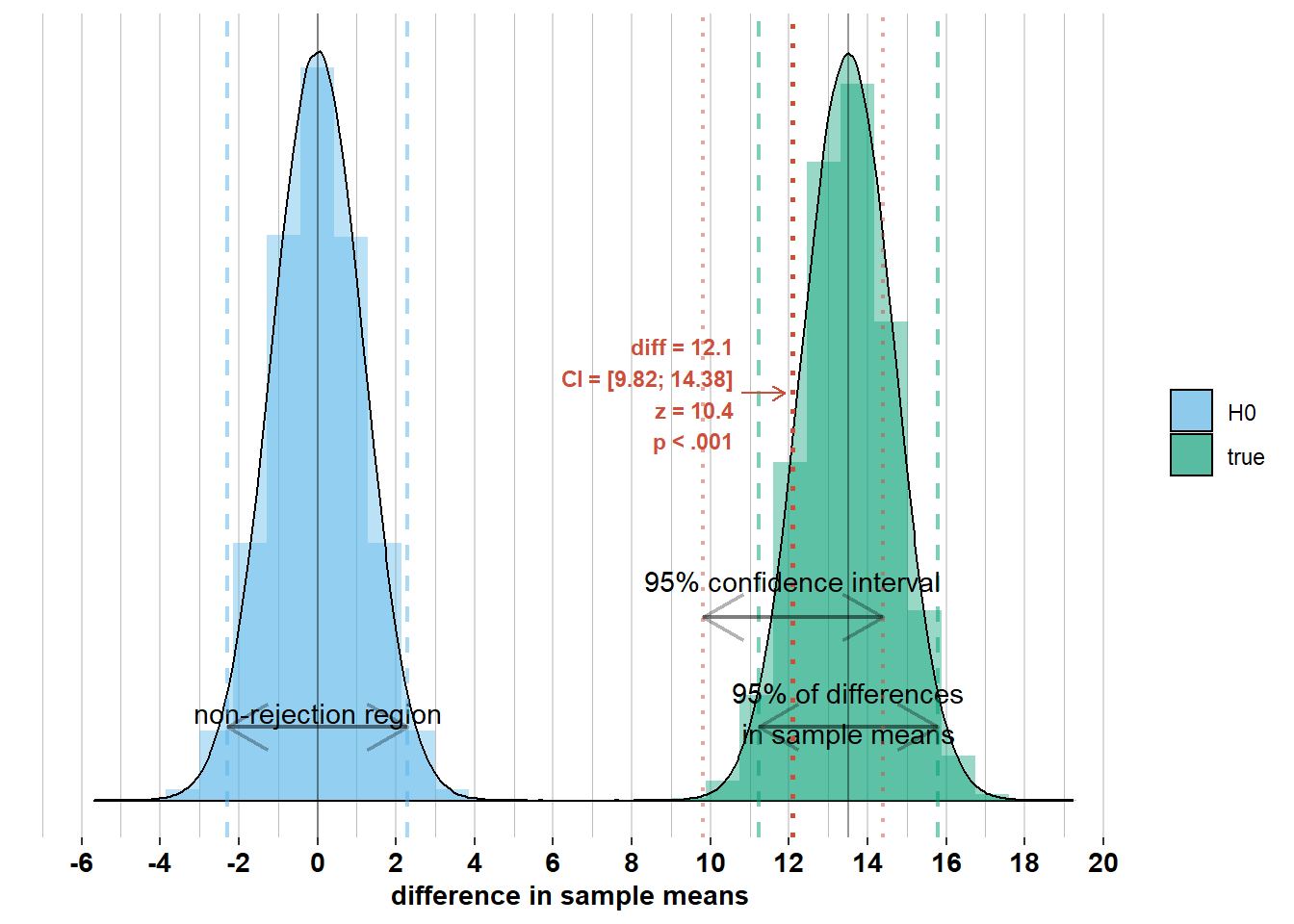
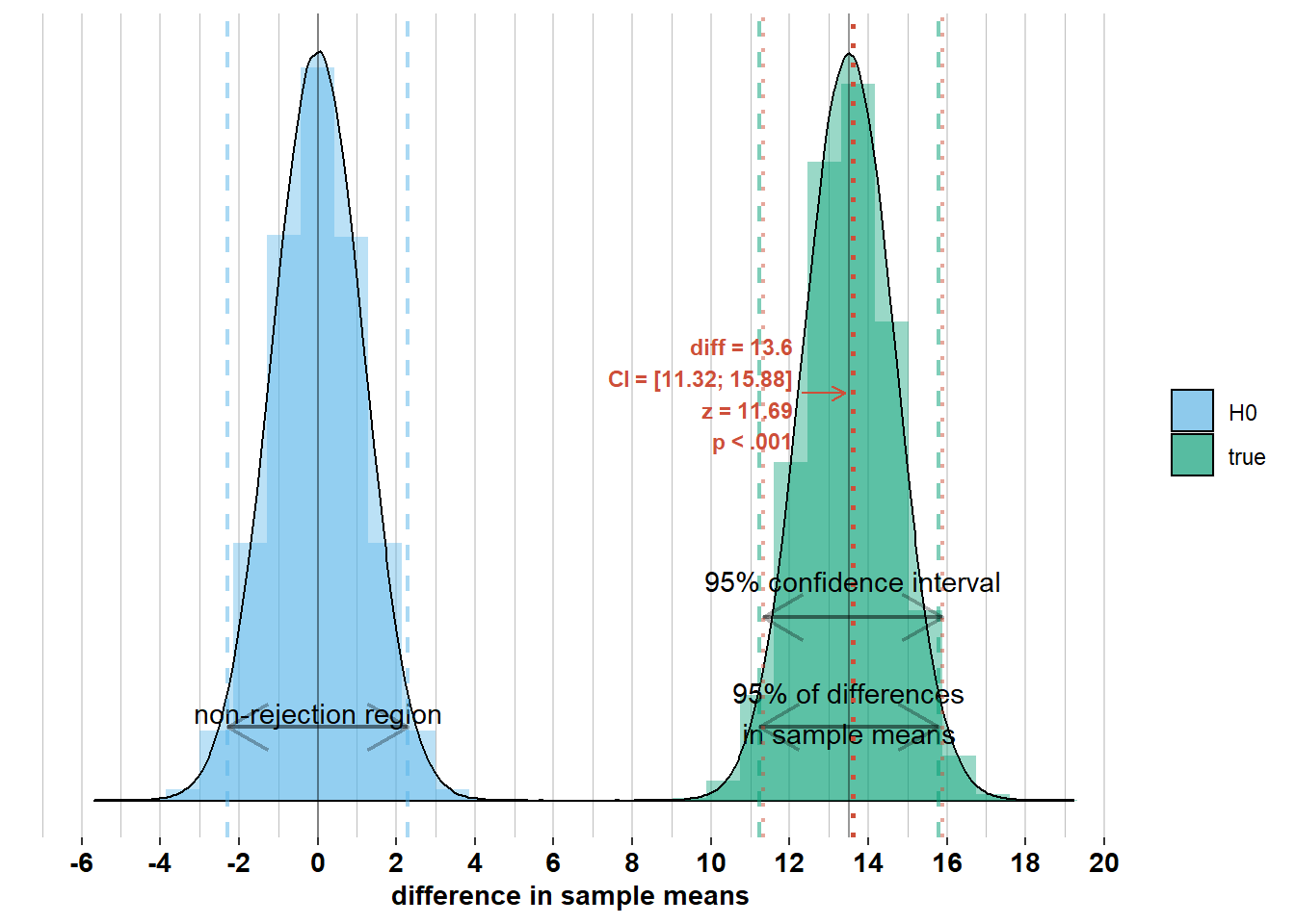
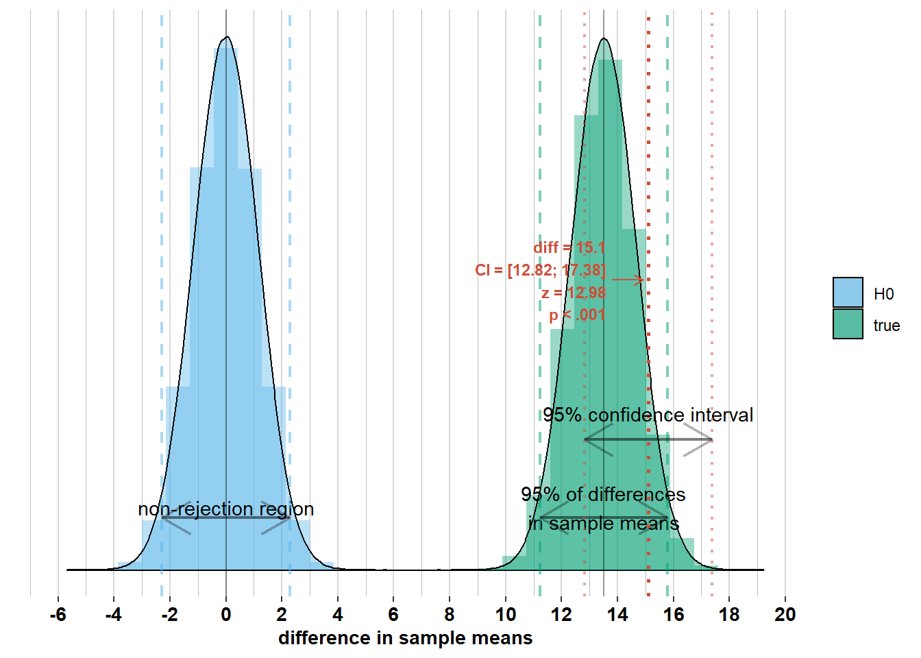
We see that for these differences in sample means, the corresponding confidence intervals do include the difference in population means. This is because they are all within the 95% interval of width \(\pm 1.96 \times\sqrt{\frac{\sigma_{men}^2}{n_{men}} + \frac{\sigma_{women}^2}{n_{women}}}\) around the difference in population means. Therefore, the confidence intervals of width \(\pm 1.96 \times\sqrt{\frac{\sigma_{men}^2}{n_{men}} + \frac{\sigma_{women}^2}{n_{women}}}\) around these differences in sample means will include the difference in population means. This brings us to the formal interpretation of the 95% confidence interval: It’s an interval that differs from survey to survey, but if you would do the survey an infinite number of times, 95% of the surveys will have a confidence interval that includes the difference in population means (because 95% of surveys will have a difference in sample means that is less than \(1.96 \times \sqrt{\frac{\sigma_{men}^2}{n_{men}} + \frac{\sigma_{women}^2}{n_{women}}}\) away from the difference in population means).
We can also use the confidence interval for rejecting \(\mathcal{H_{0}}\) or not. On the graph below you see a difference in sample means (“diff”) with a confidence interval (“CI”) that does not include zero. If zero is outside the confidence interval of width \(\pm 1.96 \times\sqrt{\frac{\sigma_{men}^2}{n_{men}} + \frac{\sigma_{women}^2}{n_{women}}}\) around the difference in sample means, then the difference in sample means is more than \(1.96 \times \sqrt{\frac{\sigma_{men}^2}{n_{men}} + \frac{\sigma_{women}^2}{n_{women}}}\) away from zero. And if the difference in sample means is more than \(1.96 \times \sqrt{\frac{\sigma_{men}^2}{n_{men}} + \frac{\sigma_{women}^2}{n_{women}}}\) away from zero, then it falls outside the non-rejection region of width \(\pm 1.96 \times\sqrt{\frac{\sigma_{men}^2}{n_{men}} + \frac{\sigma_{women}^2}{n_{women}}}\) around zero. Hence, we should reject \(\mathcal{H_{0}}\).
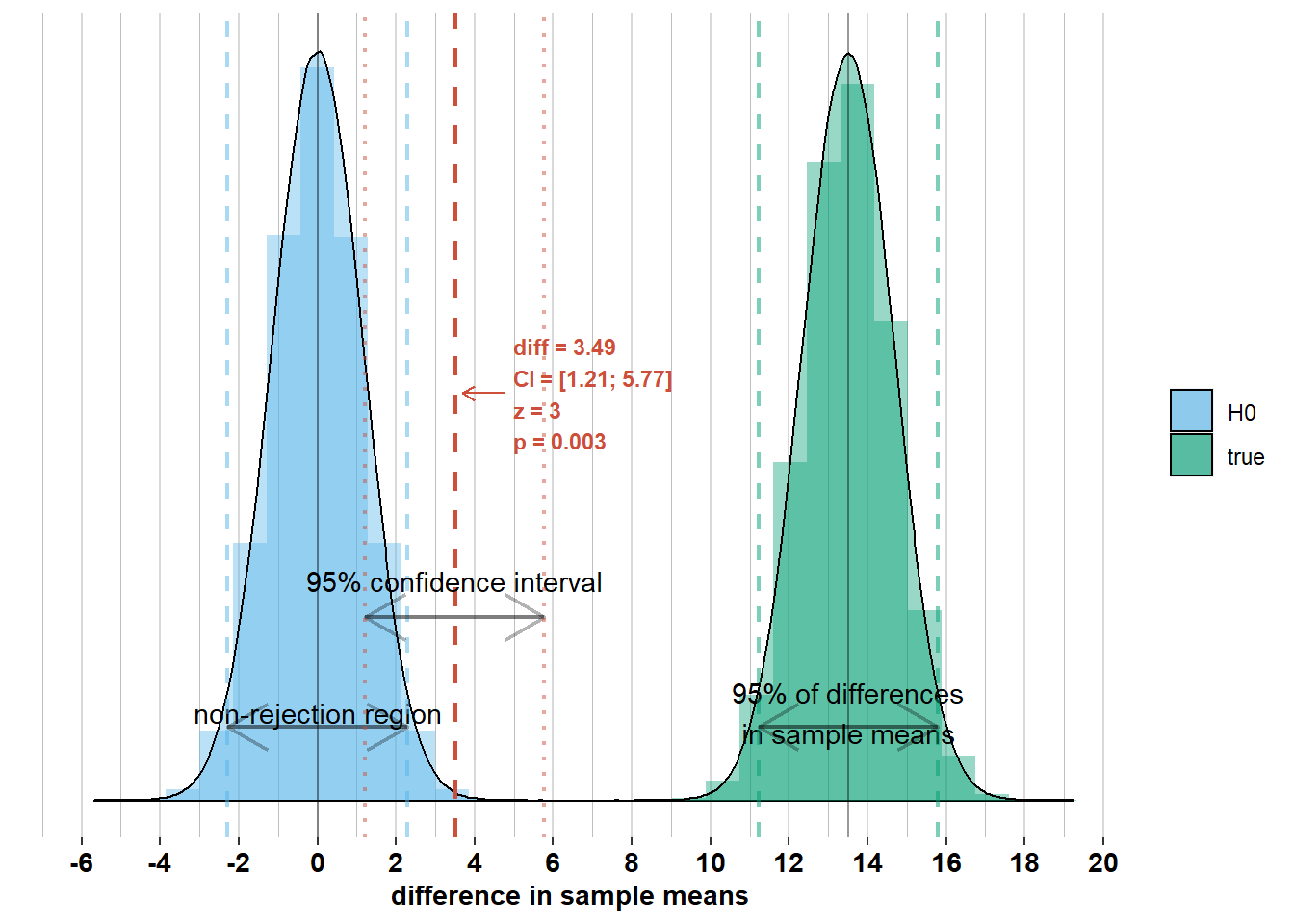
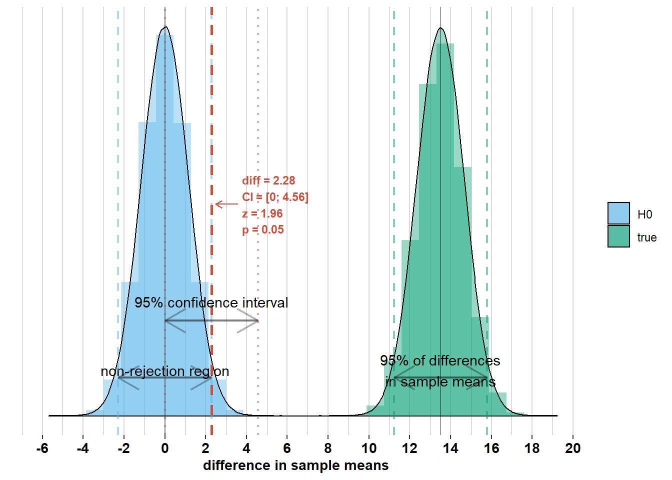
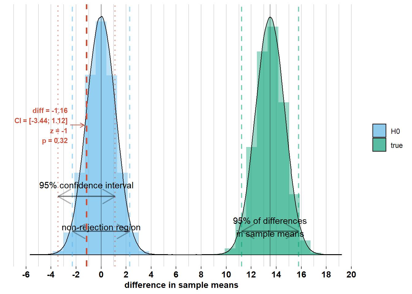
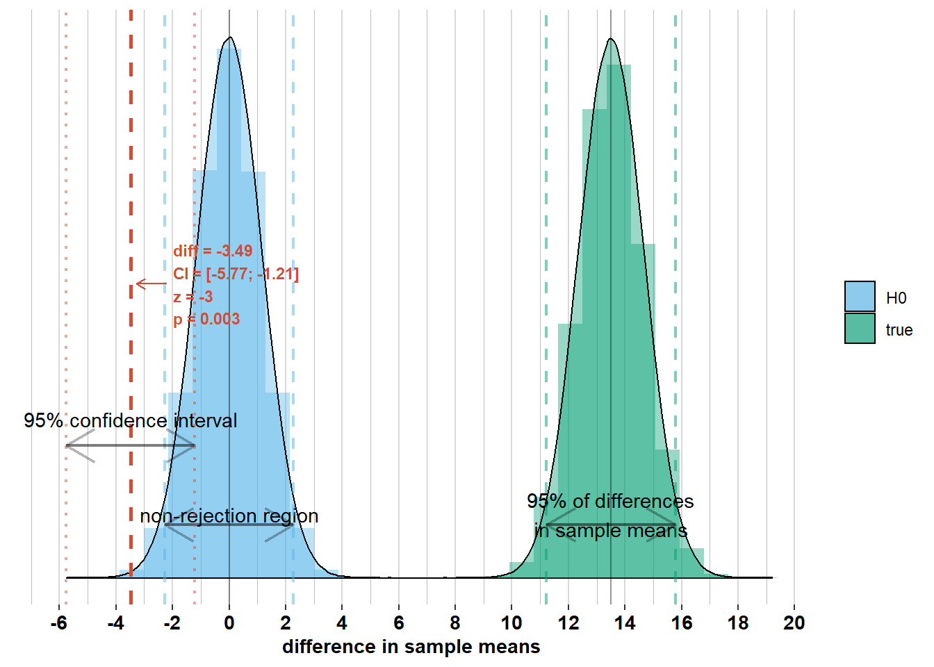
If, on the other hand, zero were within the confidence interval, then we should not have rejected \(\mathcal{H_{0}}\). Check out the graphs below where I’ve added the confidence interval to some other possible differences in sample means. Notice whether zero is inside the confidence interval or not and how this relates to Z-scores and p-values.
2.2.4 The role of the standard error
The astute reader will have noticed that there are three equivalent ways to decide whether to reject a null hypothesis:
- Method 1: transform the observed difference in sample means into a \(z\)-score and check whether this \(z\)-score is outside the non-rejection region [-1.96; 1.96],
- Method 2: calculate the p-value associated with the observed \(z\)-score and check whether it’s smaller than .05,
- Method 3: calculate a confidence interval around an observed difference in sample means and check whether the confidence interval excludes zero.
In each of these methods, the standard error, \(\sqrt{\frac{\sigma_{men}^2}{n_{men}} + \frac{\sigma_{women}^2}{n_{women}}}\), plays an important role. For methods 1 & 2, we obtain a \(z\)-score by dividing the observed difference in sample means by the standard error (\(Z = \frac{\bar{x}_{men} - \bar{x}_{women}}{\sqrt{\frac{\sigma_{men}^2}{n_{men}} + \frac{\sigma_{women}^2}{n_{women}}}}\)). For method 3, we construct a confidence interval of width \(\pm 1.96 \times\sqrt{\frac{\sigma_{men}^2}{n_{men}} + \frac{\sigma_{women}^2}{n_{women}}}\) around the observed difference in sample means, \(\bar{x}_{men} - \bar{x}_{women}\).
Additionally, we also know that in 95% of surveys, we will observe a difference in sample means inside the 95% interval around the difference in population means (\(\mu_{men} - \mu_{women}\pm 1.96 \times\sqrt{\frac{\sigma_{men}^2}{n_{men}} + \frac{\sigma_{women}^2}{n_{women}}}\)).
So, we draw an interval of width \(\pm 1.96 \times\sqrt{\frac{\sigma_{men}^2}{n_{men}} + \frac{\sigma_{women}^2}{n_{women}}}\):
- around zero to find the non-rejection region,
- around the observed difference in sample means to find the confidence interval,
- and around the difference in population means to find the interval where 95% of the differences in sample means will lie.
Let’s think about why the standard error is so important. Remember that the standard error, \(\sqrt{\frac{\sigma_{men}^2}{n_{men}} + \frac{\sigma_{women}^2}{n_{women}}}\), is the standard deviation of the sampling distribution of the difference in sample means, \(\bar{X}_{men}- \bar{X}_{women}\), which has a mean of \(\mu_{men}- \mu_{women}\). Surveys are affected by randomness, so each survey will have a different difference in sample means, \(\bar{x}_{men} - \bar{x}_{women}\). The standard deviation is the average distance, across surveys, between the differences in sample means, \(\bar{x}_{men} - \bar{x}_{women}\), and the mean of these differences, \(\mu_{men}- \mu_{women}\). In other words, it’s a measure of the degree to which the differences in sample means will vary from survey to survey.
Imagine we do a survey and observe a difference in sample means of \(\bar{x}_{men} - \bar{x}_{women}= 3\), but the standard error is quite large, say \(\sqrt{\frac{\sigma_{men}^2}{n_{men}} + \frac{\sigma_{women}^2}{n_{women}}}= 5\). In that case, we are 95% confident that the difference in population means, \(\mu_{men}- \mu_{women}\), is somewhere between \(3 \pm 1.96 \times 5 = [-6.8; 12.8]\). This confidence interval is quite wide and we cannot be sure that the difference in population means is different from zero. The difference in population means could, for example, be -6, in which case 95% of surveys will have a difference in sample means between \(-6 \pm 1.96 \times 5 = [-15.8; 3.8]\), but the difference in population means may as well be 12, in which case 95% of surveys will have a difference in sample means between \(12 \pm 1.96 \times 5 = [2.2 ; 21.8]\). There is a lot of uncertainty about the difference in population means, and if we would do the survey again, we could observe a very different difference in sample means. Therefore, the information we get from this survey is quite limited. How useful is it to know that men were 3 centimeters taller than women in a survey, if in the next repetition of this survey they could be 11 centimeters taller or even 5 centimeters shorter?
Imagine now, that we observe the same difference in sample means of \(\bar{x}_{men} - \bar{x}_{women}= 3\), but the standard error is quite small, say \(\sqrt{\frac{\sigma_{men}^2}{n_{men}} + \frac{\sigma_{women}^2}{n_{women}}}= 0.5\). In that case, we are 95% confident that the difference in population means is somewhere between \(3 \pm 1.96 \times 0.5 = [2.02; 3.98]\). This confidence interval is quite narrow and we can be relatively sure that the difference in population means is different from zero. The difference in population means could, for example, be 2.1, in which case 95% of surveys will have a difference in sample means between \(2.1 \pm 1.96 \times 0.5 = [1.12; 3.08]\), or the difference in population means could be 3.9, in which case 95% of surveys will have a difference in sample means between \(3.9 \pm 1.96 \times 0.5 = [2.92 ; 4.88]\). Compared to the case where the standard error was equal to 5, there is much less uncertainty about the difference in population means. If we would do this survey again, we would observe a difference in sample means that is quite similar to the one that we have observed the first time. Therefore, this survey is much more informative than the survey with standard error equal to 5, where the result could change quite a bit from one survey to the next.
So we see that, depending on the standard error, the same difference in sample means provides different degrees of certainty about the difference in population means. The \(Z\)-score, which is the ratio of the difference in sample means versus the standard error, captures this certainty, or better, uncertainty. In essence, every statistical test is a ratio of signal (difference) versus noise (variation). The higher this ratio, the more certainty we have about our statistical inferences. Let’s now think about how we can reduce the standard error when collecting data.
2.2.5 The two components of the standard error: \(\sigma\) and \(\mathcal{n}\)
If we look at the formula of the standard error, \(\sqrt{\frac{\sigma_{men}^2}{n_{men}} + \frac{\sigma_{women}^2}{n_{women}}}\), we see that it has two components:
- the \(\sigma\)’s are the standard deviations of our two populations
- the \(\mathcal{n}\)’s are the sizes of our two samples
In the example of height of men and women, the \(\sigma\)’s represent the variation in height among the population of men and among the population of women. These population standard deviations are unknown to us (we will address this issue in section 2.4). Also, these standard deviations are not under our control: we cannot affect the variation in height among men and women.
The \(\mathcal{n}\)’s represent the sizes of our samples and are under our control. In theory, we can choose whether we include less or more respondents in our surveys (in reality, of course, there are constraints on our time and money). The larger the sample sizes, the larger the denominator of the standard error and hence the smaller the standard error. This means that for a given difference in sample means, smaller standard errors mean larger \(Z\)-scores, smaller p-values, and narrower confidence intervals. In other words, we are more likely to reject the null hypothesis with larger sample sizes.