Chapter 9 Practical Sheet Solutions
9.1 Practical 1
9.1.1 Load and visualise the data
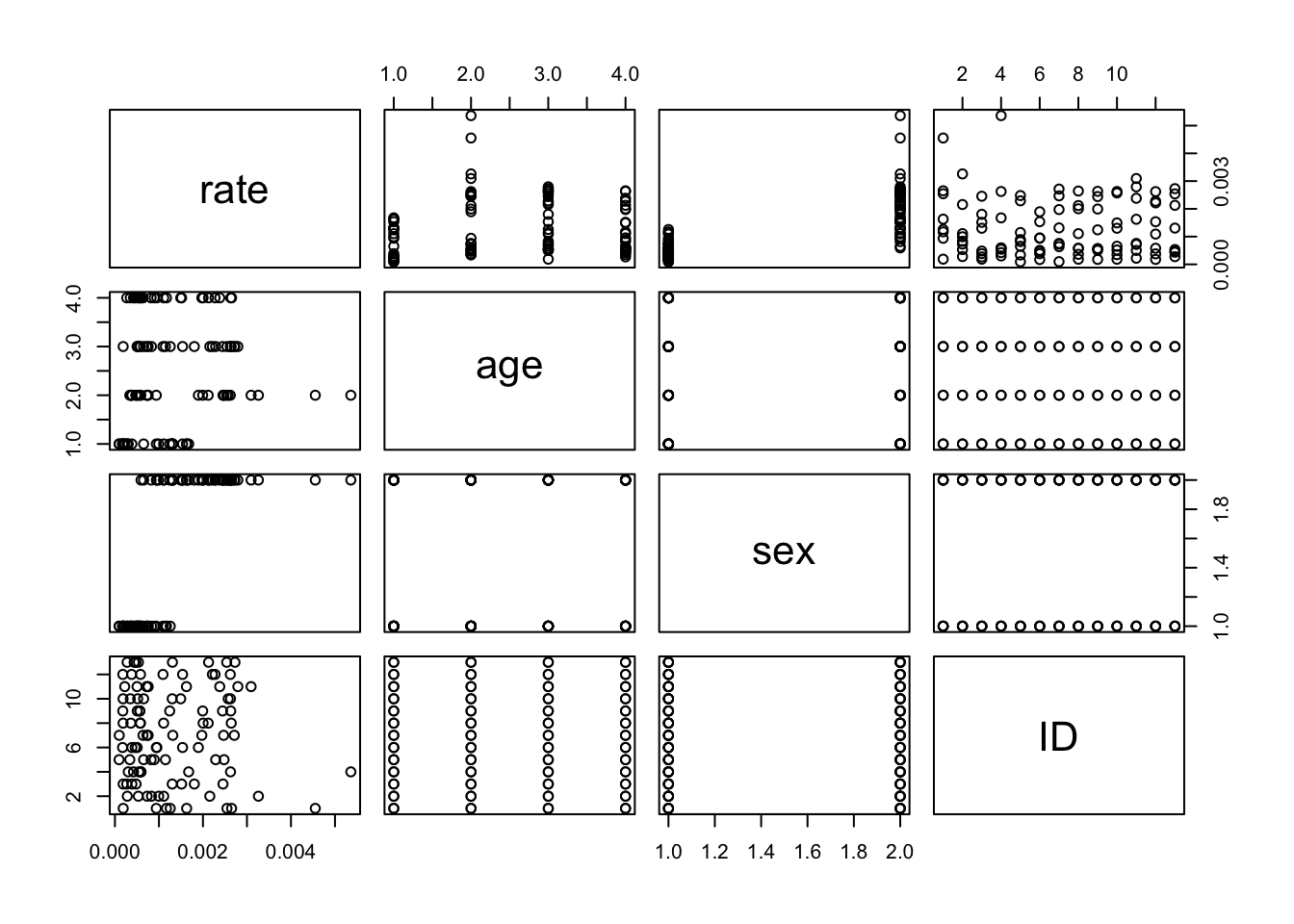
Load the data, inspect its contents, and plot all pairs of variables against each other.
##   Taste Acetic  H2S Lactic
## 1  12.3     94   23   0.86
## 2  20.9    174  155   1.53
## 3  39.0    214  230   1.57
## 4  47.9    317 1801   1.81
## 5   5.6    106   45   0.99
## 6  25.9    298 2000   1.09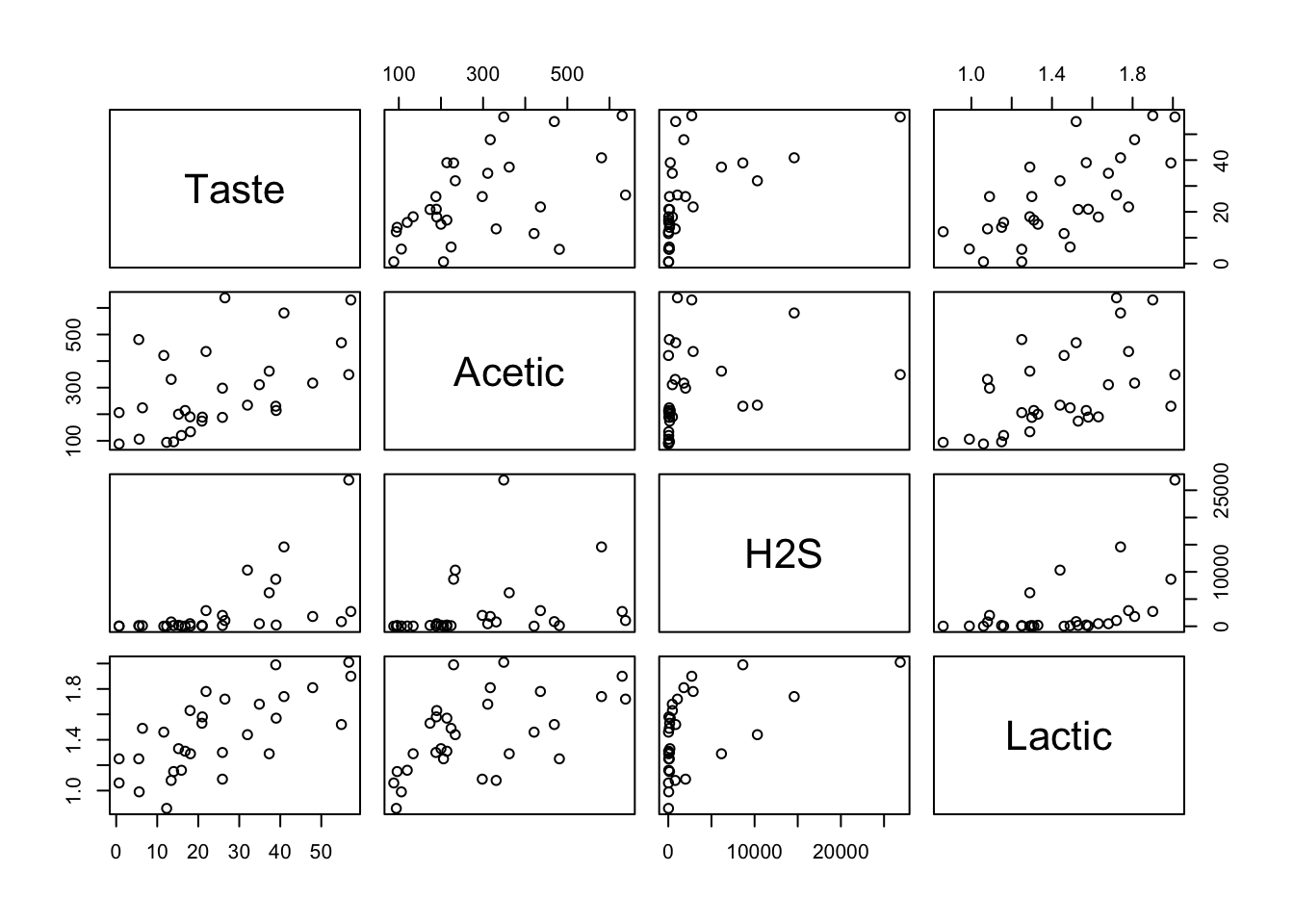
From the plot, it seems Lactic could have some good linear correlation with Taste.
We compute and check the correlation matrix to confirm.
##            Taste    Acetic       H2S    Lactic
## Taste  1.0000000 0.5131983 0.5604809 0.7042362
## Acetic 0.5131983 1.0000000 0.2824617 0.5410837
## H2S    0.5604809 0.2824617 1.0000000 0.5075128
## Lactic 0.7042362 0.5410837 0.5075128 1.0000000
9.1.2 Gaussian GLM and linear model
We first fit a linear model to the data and check its summary.
##
## Call:
## lm(formula = Taste ~ ., data = cheese)
##
## Residuals:
##     Min      1Q  Median      3Q     Max
## -16.208  -7.266  -1.652   7.385  26.338
##
## Coefficients:
##               Estimate Std. Error t value Pr(>|t|)
## (Intercept) -1.898e+01  1.127e+01  -1.684   0.1042
## Acetic       1.890e-02  1.563e-02   1.210   0.2373
## H2S          7.668e-04  4.188e-04   1.831   0.0786 .
## Lactic       2.501e+01  9.062e+00   2.760   0.0105 *
## ---
## Signif. codes:  0 '***' 0.001 '**' 0.01 '*' 0.05 '.' 0.1 ' ' 1
##
## Residual standard error: 11.19 on 26 degrees of freedom
## Multiple R-squared:  0.5754, Adjusted R-squared:  0.5264
## F-statistic: 11.74 on 3 and 26 DF,  p-value: 4.748e-05
Now we fit a Gaussian GLM with the identity link function and check its summary. Note that we do not need to specify the family parameter here because the Gaussian family with identity link is the default option for glm.
##
## Call:
## glm(formula = Taste ~ ., data = cheese)
##
## Coefficients:
##               Estimate Std. Error t value Pr(>|t|)
## (Intercept) -1.898e+01  1.127e+01  -1.684   0.1042
## Acetic       1.890e-02  1.563e-02   1.210   0.2373
## H2S          7.668e-04  4.188e-04   1.831   0.0786 .
## Lactic       2.501e+01  9.062e+00   2.760   0.0105 *
## ---
## Signif. codes:  0 '***' 0.001 '**' 0.01 '*' 0.05 '.' 0.1 ' ' 1
##
## (Dispersion parameter for gaussian family taken to be 125.1432)
##
##     Null deviance: 7662.9  on 29  degrees of freedom
## Residual deviance: 3253.7  on 26  degrees of freedom
## AIC: 235.73
##
## Number of Fisher Scoring iterations: 2
The summaries show that the two models have the same coefficients. The p-value for Lactic is less than 0.05.
Now we compute the RSS and then the residual standard error.
## [1] 11.18674Next, we compute the R-squared.
meanTaste <- mean(cheese$Taste)
tss <- sum((cheese$Taste - meanTaste)^2)
rSquared <- 1 - rss/tss
rSquared
## [1] 0.5753921We also compute the adjusted R-squared.
## [1] 0.5263989The last three results should be similar to those in the linear model’s summary.
Finally, we compute the estimated dispersion. This should give the same number as in the GLM model summary.
## [1] 125.1432Note that we can also get the estimated dispersion from a GLM model summary using:
## [1] 125.14329.1.3 Gamma GLMs
We fit a Gamma GLM with inverse link (the default link).
##
## Call:
## glm(formula = Taste ~ ., family = Gamma, data = cheese)
##
## Coefficients:
##               Estimate Std. Error t value Pr(>|t|)
## (Intercept)  1.289e-01  2.729e-02   4.726 6.94e-05 ***
## Acetic      -2.827e-05  2.478e-05  -1.141   0.2644
## H2S         -1.641e-07  4.896e-07  -0.335   0.7402
## Lactic      -4.933e-02  1.883e-02  -2.620   0.0145 *
## ---
## Signif. codes:  0 '***' 0.001 '**' 0.01 '*' 0.05 '.' 0.1 ' ' 1
##
## (Dispersion parameter for Gamma family taken to be 0.3188002)
##
##     Null deviance: 21.104  on 29  degrees of freedom
## Residual deviance: 14.664  on 26  degrees of freedom
## AIC: 246.99
##
## Number of Fisher Scoring iterations: 5
Then we estimate the dispersion for this model.
## [1] 0.3187877Similarly, we fit a Gamma GLM with log link and estimate its dispersion.
##
## Call:
## glm(formula = Taste ~ ., family = Gamma(link = log), data = cheese)
##
## Coefficients:
##              Estimate Std. Error t value Pr(>|t|)
## (Intercept) 1.137e+00  5.412e-01   2.101   0.0455 *
## Acetic      9.005e-04  7.505e-04   1.200   0.2410
## H2S         2.126e-05  2.011e-05   1.057   0.3003
## Lactic      1.130e+00  4.353e-01   2.597   0.0153 *
## ---
## Signif. codes:  0 '***' 0.001 '**' 0.01 '*' 0.05 '.' 0.1 ' ' 1
##
## (Dispersion parameter for Gamma family taken to be 0.2886981)
##
##     Null deviance: 21.104  on 29  degrees of freedom
## Residual deviance: 13.922  on 26  degrees of freedom
## AIC: 245.31
##
## Number of Fisher Scoring iterations: 6## [1] 0.2886981The two dispersion estimates should be similar (or very close) to the numbers printed in the model summaries (equivalently, the ones printed below).
## [1] 0.3188002## [1] 0.28869819.1.4 Fisher information matrices
To compute the Fisher information matrix for model2, we first compute the covariance matrix of its estimated parameters.
##               (Intercept)        Acetic           H2S        Lactic
## (Intercept) 126.968392322  2.906005e-02  1.952093e-03 -94.543244249
## Acetic        0.029060047  2.441794e-04 -7.093845e-08  -0.068138650
## H2S           0.001952093 -7.093845e-08  1.753887e-07  -0.001668523
## Lactic      -94.543244249 -6.813865e-02 -1.668523e-03  82.119275850
We can check that the diagonal of this matrix is the square of the standard error column in the model summary.
##  (Intercept)       Acetic          H2S       Lactic
## 1.269684e+02 2.441794e-04 1.753887e-07 8.211928e+01
Now we inverse f2_inv to obtain the Fisher information matrix.
##             (Intercept)       Acetic          H2S       Lactic
## (Intercept)   0.2397254     68.12198     647.9779    0.3456841
## Acetic       68.1219806  25149.38068  243706.4456  104.2477262
## H2S         647.9778779 243706.44562 9432054.4333 1139.8707583
## Lactic        0.3456841    104.24773    1139.8708    0.5198207
We can do the same for model3 and model4 but using another (equivalent) way to get the covariance matrices.
##              (Intercept)       Acetic          H2S       Lactic
## (Intercept)     72523.97     28174463 5.592281e+08     124745.8
## Acetic       28174463.36  13029598379 2.158724e+11   49722197.5
## H2S         559228082.05 215872392263 1.132172e+13 1077030620.5
## Lactic 124745.79 49722198 1.077031e+09 220072.3## (Intercept) Acetic H2S Lactic
## (Intercept) 103.9148 29529.12 280881.7 149.8451
## Acetic 29529.1193 10901607.03 105640450.4 45188.6971
## H2S 280881.6758 105640450.36 4088552010.0 494104.5361
## Lactic 149.8451 45188.70 494104.5 225.32889.1.5 Models without the intercept
Note that if we want to fit a model without the intercept, we can add + 0 or - 1 to the formula of glm. For instance,
##
## Call:
## glm(formula = Taste ~ . + 0, data = cheese)
##
## Coefficients:
##         Estimate Std. Error t value Pr(>|t|)
## Acetic  0.023246   0.015927   1.460  0.15596
## H2S     0.001059   0.000394   2.686  0.01220 *
## Lactic 10.880532   3.537987   3.075  0.00477 **
## ---
## Signif. codes:  0 '***' 0.001 '**' 0.01 '*' 0.05 '.' 0.1 ' ' 1
##
## (Dispersion parameter for gaussian family taken to be 133.6519)
##
##     Null deviance: 25719.4  on 30  degrees of freedom
## Residual deviance:  3608.6  on 27  degrees of freedom
## AIC: 236.83
##
## Number of Fisher Scoring iterations: 2
or
##
## Call:
## glm(formula = Taste ~ . - 1, data = cheese)
##
## Coefficients:
##         Estimate Std. Error t value Pr(>|t|)
## Acetic  0.023246   0.015927   1.460  0.15596
## H2S     0.001059   0.000394   2.686  0.01220 *
## Lactic 10.880532   3.537987   3.075  0.00477 **
## ---
## Signif. codes:  0 '***' 0.001 '**' 0.01 '*' 0.05 '.' 0.1 ' ' 1
##
## (Dispersion parameter for gaussian family taken to be 133.6519)
##
##     Null deviance: 25719.4  on 30  degrees of freedom
## Residual deviance:  3608.6  on 27  degrees of freedom
## AIC: 236.83
##
## Number of Fisher Scoring iterations: 2
We fit a linear model and compare:
##
## Call:
## lm(formula = Taste ~ . + 0, data = cheese)
##
## Residuals:
##      Min       1Q   Median       3Q      Max
## -19.4090  -7.5079  -0.7735   4.4359  26.5531
##
## Coefficients:
##         Estimate Std. Error t value Pr(>|t|)
## Acetic  0.023246   0.015927   1.460  0.15596
## H2S     0.001059   0.000394   2.686  0.01220 *
## Lactic 10.880532   3.537987   3.075  0.00477 **
## ---
## Signif. codes:  0 '***' 0.001 '**' 0.01 '*' 0.05 '.' 0.1 ' ' 1
##
## Residual standard error: 11.56 on 27 degrees of freedom
## Multiple R-squared:  0.8597, Adjusted R-squared:  0.8441
## F-statistic: 55.15 on 3 and 27 DF,  p-value: 1.215e-11
We can compute the residual standard error, R-squared, adjusted R-squared, dispersion, and Fisher information matrix as before. However, note that the TSS has a slightly different formula when there is no intercept. In this case, \(TSS = \sum y_i^2\) since the null model without the intercept will now return 0 instead of \(\bar{y}\).
## [1] 11.56079## [1] 0.8596935## [1] 0.8441039## [1] 133.6519## Acetic H2S Lactic
## Acetic 23548.28664 228191.275 97.6109658
## H2S 228191.27473 8831578.168 1067.3027572
## Lactic 97.61097 1067.303 0.4867271Similarly, we can do the same for the Gamma GLMs.
##
## Call:
## glm(formula = Taste ~ . - 1, family = Gamma, data = cheese)
##
## Coefficients:
##          Estimate Std. Error t value Pr(>|t|)
## Acetic -5.058e-05  3.511e-05  -1.441  0.16115
## H2S    -1.851e-06  5.968e-07  -3.101  0.00448 **
## Lactic  4.218e-02  9.459e-03   4.459  0.00013 ***
## ---
## Signif. codes:  0 '***' 0.001 '**' 0.01 '*' 0.05 '.' 0.1 ' ' 1
##
## (Dispersion parameter for Gamma family taken to be 0.5713799)
##
##     Null deviance:   NaN  on 30  degrees of freedom
## Residual deviance: 22.99  on 27  degrees of freedom
## AIC: 259.82
##
## Number of Fisher Scoring iterations: 6## [1] 0.5713799## Acetic H2S Lactic
## Acetic 6140076654 1.245799e+11 23096661.4
## H2S 124579869304 5.863372e+12 552378685.7
## Lactic 23096661 5.523787e+08 100161.6##
## Call:
## glm(formula = Taste ~ . - 1, family = Gamma(link = log), data = cheese)
##
## Coefficients:
## Estimate Std. Error t value Pr(>|t|)
## Acetic 6.779e-04 8.834e-04 0.767 0.449
## H2S 6.072e-06 2.185e-05 0.278 0.783
## Lactic 1.978e+00 1.962e-01 10.081 1.19e-10 ***
## ---
## Signif. codes: 0 '***' 0.001 '**' 0.01 '*' 0.05 '.' 0.1 ' ' 1
##
## (Dispersion parameter for Gamma family taken to be 0.4111806)
##
## Null deviance: 1241.102 on 30 degrees of freedom
## Residual deviance: 15.318 on 27 degrees of freedom
## AIC: 246.4
##
## Number of Fisher Scoring iterations: 6## [1] 0.4111806## Acetic H2S Lactic
## Acetic 7654235.40 74172264.0 31727.8841
## H2S 74172263.96 2870653787.1 346920.6345
## Lactic 31727.88 346920.6 158.20799.2 Practical 2
9.2.2 Rescaled binomial logit model
Fit the model
We fit the model using proportions and weights.
##
## Call:
## glm(formula = rate ~ age + sex, family = binomial(), data = irlsuicide,
##     weights = pop)
##
## Coefficients:
##             Estimate Std. Error z value Pr(>|z|)
## (Intercept) -8.20113    0.04350 -188.54   <2e-16 ***
## age2         0.77204    0.04544   16.99   <2e-16 ***
## age3         0.72841    0.04056   17.96   <2e-16 ***
## age4         0.50190    0.04936   10.17   <2e-16 ***
## sex1         1.44616    0.04094   35.33   <2e-16 ***
## ---
## Signif. codes:  0 '***' 0.001 '**' 0.01 '*' 0.05 '.' 0.1 ' ' 1
##
## (Dispersion parameter for binomial family taken to be 1)
##
##     Null deviance: 2301.66  on 103  degrees of freedom
## Residual deviance:  291.29  on  99  degrees of freedom
## AIC: 803.94
##
## Number of Fisher Scoring iterations: 4
We can also fit the model using numbers of deaths and non-deaths. Note that here we do not set the weights argument. The summaries of the two models should be the same.
irlsuicide$notdead <- irlsuicide$pop - irlsuicide$death

glm2 <- glm(cbind(death, notdead) ~ age + sex,
            data = irlsuicide, family = binomial())
summary(glm2)
##
## Call:
## glm(formula = cbind(death, notdead) ~ age + sex, family = binomial(),
## data = irlsuicide)
##
## Coefficients:
## Estimate Std. Error z value Pr(>|z|)
## (Intercept) -8.20113 0.04350 -188.54 <2e-16 ***
## age2 0.77204 0.04544 16.99 <2e-16 ***
## age3 0.72841 0.04056 17.96 <2e-16 ***
## age4 0.50190 0.04936 10.17 <2e-16 ***
## sex1 1.44616 0.04094 35.33 <2e-16 ***
## ---
## Signif. codes: 0 '***' 0.001 '**' 0.01 '*' 0.05 '.' 0.1 ' ' 1
##
## (Dispersion parameter for binomial family taken to be 1)
##
## Null deviance: 2301.66 on 103 degrees of freedom
## Residual deviance: 291.29 on 99 degrees of freedom
## AIC: 803.94
##
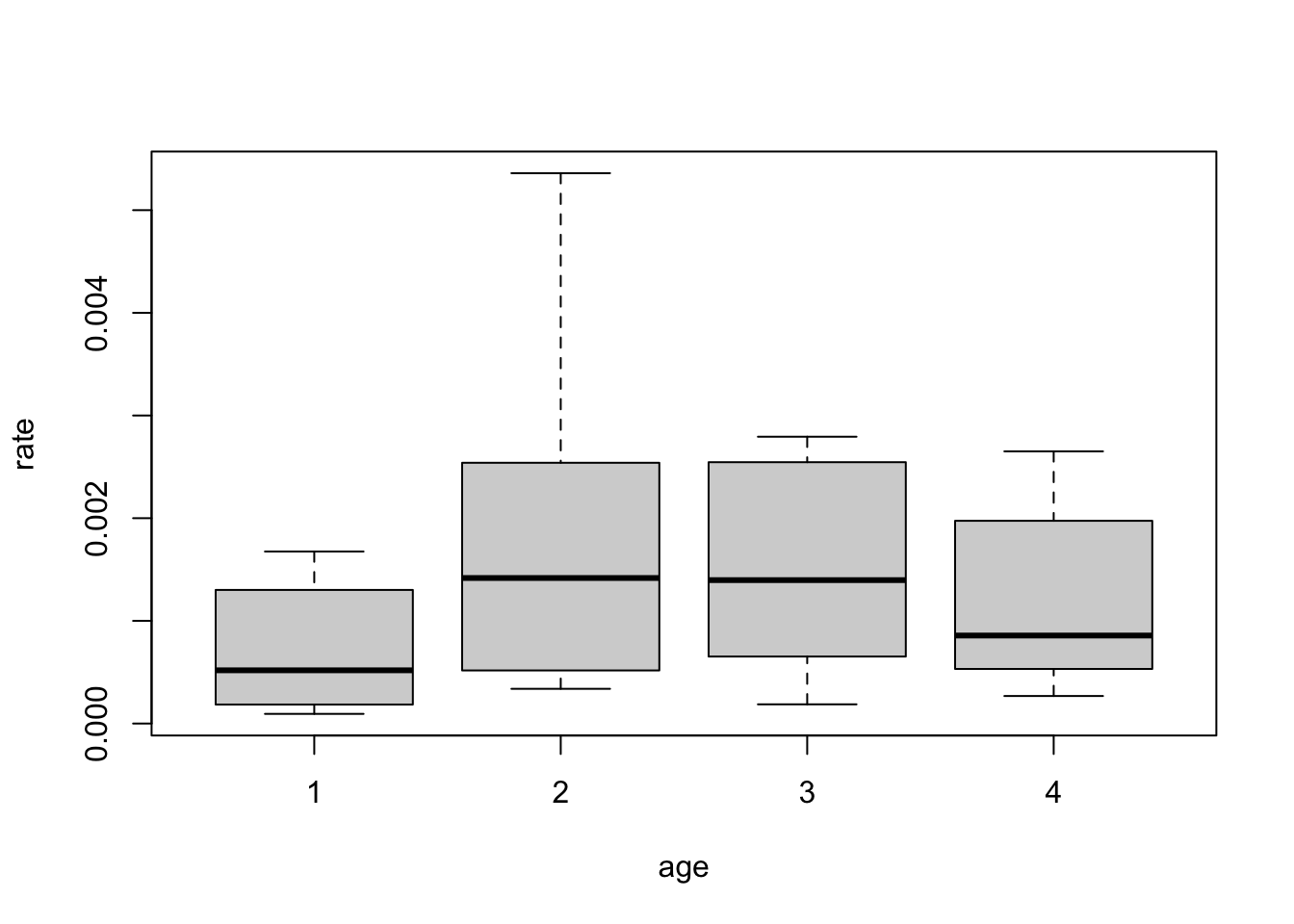
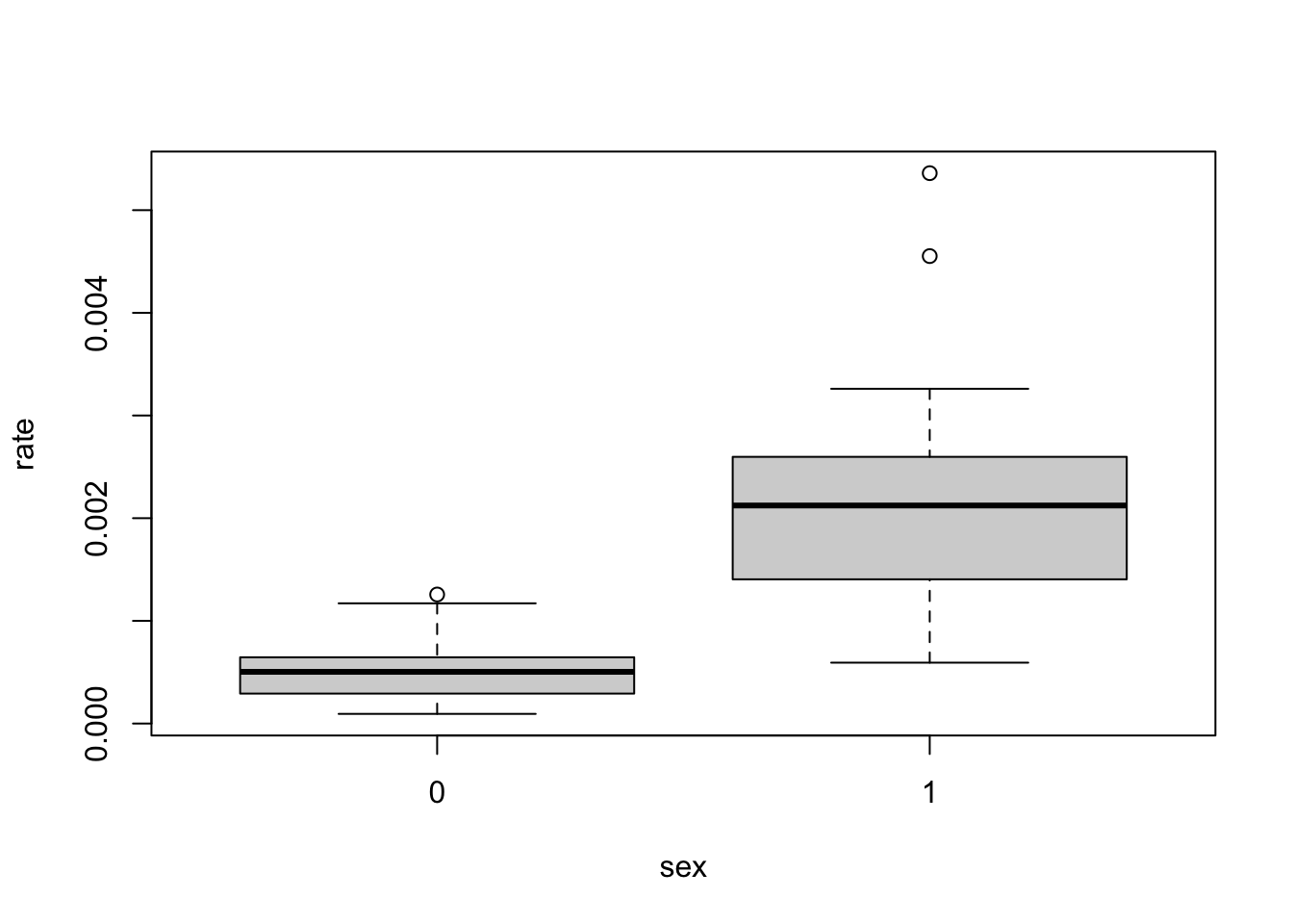
## Number of Fisher Scoring iterations: 4Interpret the model
The parameter value for \(\texttt{sex1}\) is 1.45, which is greater than 0. This means that, according to the model, males (\(\texttt{sex} = 1\)) have higher death rate than females. Note that here, \(\texttt{sex} = 0\) is used as a reference (value 0). Similarly, for the \(\texttt{age}\) covariate, age group 1 is used as a reference and has value 0. The estimated parameters for \(\texttt{age} = 2, 3, 4\) are all greater than 0, indicating that these groups have higher death rates than group 1. According to the model, age group 2 has the highest rate (parameter value 0.77), followed by group 3 (0.73), then group 4 (0.50), and finally group 1 (0).
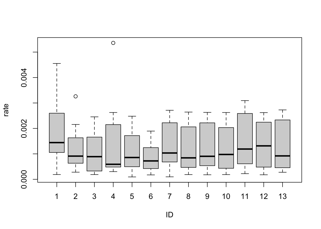
Include region IDs
We include the region IDs into the model.
glm3 <- glm(rate~age + sex + ID, weights = pop,
            data = irlsuicide, family = binomial())
summary(glm3)
##
## Call:
## glm(formula = rate ~ age + sex + ID, family = binomial(), data = irlsuicide,
## weights = pop)
##
## Coefficients:
## Estimate Std. Error z value Pr(>|z|)
## (Intercept) -7.83022 0.08297 -94.371 < 2e-16 ***
## age2 0.77568 0.04544 17.069 < 2e-16 ***
## age3 0.72427 0.04057 17.851 < 2e-16 ***
## age4 0.47303 0.04948 9.561 < 2e-16 ***
## sex1 1.44189 0.04095 35.213 < 2e-16 ***
## ID2 -0.38530 0.08584 -4.488 7.18e-06 ***
## ID3 -0.43499 0.15794 -2.754 0.005884 **
## ID4 -0.14573 0.14233 -1.024 0.305905
## ID5 -0.55167 0.18199 -3.031 0.002434 **
## ID6 -0.69006 0.08349 -8.266 < 2e-16 ***
## ID7 -0.29398 0.09268 -3.172 0.001513 **
## ID8 -0.39606 0.10003 -3.959 7.52e-05 ***
## ID9 -0.34822 0.09127 -3.815 0.000136 ***
## ID10 -0.36341 0.09868 -3.683 0.000231 ***
## ID11 -0.15210 0.08645 -1.759 0.078506 .
## ID12 -0.24432 0.08526 -2.866 0.004161 **
## ID13 -0.29089 0.09057 -3.212 0.001320 **
## ---
## Signif. codes: 0 '***' 0.001 '**' 0.01 '*' 0.05 '.' 0.1 ' ' 1
##
## (Dispersion parameter for binomial family taken to be 1)
##
## Null deviance: 2301.66 on 103 degrees of freedom
## Residual deviance: 163.24 on 87 degrees of freedom
## AIC: 699.9
##
## Number of Fisher Scoring iterations: 4We can also use the \(\texttt{Region}\) variable instead of \(\texttt{ID}\) since they are basically the same.
glm4 <- glm(rate ~ age + sex + Region, weights = pop,
data = irlsuicide, family = binomial())
summary(glm4)##
## Call:
## glm(formula = rate ~ age + sex + Region, family = binomial(),
## data = irlsuicide, weights = pop)
##
## Coefficients:
## Estimate Std. Error z value Pr(>|z|)
## (Intercept) -7.83022 0.08297 -94.371 < 2e-16 ***
## age2 0.77568 0.04544 17.069 < 2e-16 ***
## age3 0.72427 0.04057 17.851 < 2e-16 ***
## age4 0.47303 0.04948 9.561 < 2e-16 ***
## sex1 1.44189 0.04095 35.213 < 2e-16 ***
## RegionDublin -0.38530 0.08584 -4.488 7.18e-06 ***
## RegionEHB - Dub. -0.69006 0.08349 -8.266 < 2e-16 ***
## RegionGalway -0.43499 0.15794 -2.754 0.005884 **
## RegionLim. -0.14573 0.14233 -1.024 0.305905
## RegionMid HB -0.39606 0.10003 -3.959 7.52e-05 ***
## RegionMWHB - Lim. -0.29398 0.09268 -3.172 0.001513 **
## RegionNEHB -0.34822 0.09127 -3.815 0.000136 ***
## RegionNWHB -0.36341 0.09868 -3.683 0.000231 ***
## RegionSEHB - Wat. -0.15210 0.08645 -1.759 0.078506 .
## RegionSHB - Cork -0.24432 0.08526 -2.866 0.004161 **
## RegionWaterf. -0.55167 0.18199 -3.031 0.002434 **
## RegionWHB - Gal. -0.29089 0.09057 -3.212 0.001320 **
## ---
## Signif. codes: 0 '***' 0.001 '**' 0.01 '*' 0.05 '.' 0.1 ' ' 1
##
## (Dispersion parameter for binomial family taken to be 1)
##
## Null deviance: 2301.66 on 103 degrees of freedom
## Residual deviance: 163.24 on 87 degrees of freedom
## AIC: 699.9
##
## Number of Fisher Scoring iterations: 4From the summary, ID4 and ID11 are the least significant. The others are significant at 1%, some at much higher levels.
Make prediction
We can make the prediction using either model above. Note that we need an extra space in \(\texttt{`Galway '}\) for the glm4 code to work.
## 1
## 0.002239986## 1
## 0.0022399869.2.3 Rescaled Poisson model
Fit the model
glm_poi <- glm(death ~ age + sex, offset = log(pop),
data = irlsuicide, family = poisson())
summary(glm_poi)##
## Call:
## glm(formula = death ~ age + sex, family = poisson(), data = irlsuicide,
## offset = log(pop))
##
## Coefficients:
## Estimate Std. Error z value Pr(>|z|)
## (Intercept) -8.20092 0.04348 -188.61 <2e-16 ***
## age2 0.77089 0.04540 16.98 <2e-16 ***
## age3 0.72734 0.04053 17.95 <2e-16 ***
## age4 0.50125 0.04932 10.16 <2e-16 ***
## sex1 1.44468 0.04092 35.30 <2e-16 ***
## ---
## Signif. codes: 0 '***' 0.001 '**' 0.01 '*' 0.05 '.' 0.1 ' ' 1
##
## (Dispersion parameter for poisson family taken to be 1)
##
## Null deviance: 2299.12 on 103 degrees of freedom
## Residual deviance: 290.97 on 99 degrees of freedom
## AIC: 803.76
##
## Number of Fisher Scoring iterations: 4Include regions IDs
glm_poi1 <- glm(death ~ age + sex + ID, offset = log(pop),
data = irlsuicide, family = poisson())
summary(glm_poi1)##
## Call:
## glm(formula = death ~ age + sex + ID, family = poisson(), data = irlsuicide,
## offset = log(pop))
##
## Coefficients:
## Estimate Std. Error z value Pr(>|z|)
## (Intercept) -7.83067 0.08290 -94.463 < 2e-16 ***
## age2 0.77447 0.04540 17.057 < 2e-16 ***
## age3 0.72317 0.04054 17.838 < 2e-16 ***
## age4 0.47240 0.04944 9.555 < 2e-16 ***
## sex1 1.44036 0.04093 35.190 < 2e-16 ***
## ID2 -0.38456 0.08575 -4.485 7.31e-06 ***
## ID3 -0.43418 0.15781 -2.751 0.005936 **
## ID4 -0.14541 0.14218 -1.023 0.306439
## ID5 -0.55068 0.18185 -3.028 0.002460 **
## ID6 -0.68890 0.08340 -8.260 < 2e-16 ***
## ID7 -0.29339 0.09258 -3.169 0.001529 **
## ID8 -0.39530 0.09993 -3.956 7.63e-05 ***
## ID9 -0.34754 0.09117 -3.812 0.000138 ***
## ID10 -0.36270 0.09858 -3.679 0.000234 ***
## ID11 -0.15178 0.08635 -1.758 0.078798 .
## ID12 -0.24382 0.08516 -2.863 0.004197 **
## ID13 -0.29030 0.09048 -3.209 0.001334 **
## ---
## Signif. codes: 0 '***' 0.001 '**' 0.01 '*' 0.05 '.' 0.1 ' ' 1
##
## (Dispersion parameter for poisson family taken to be 1)
##
## Null deviance: 2299.12 on 103 degrees of freedom
## Residual deviance: 163.13 on 87 degrees of freedom
## AIC: 699.92
##
## Number of Fisher Scoring iterations: 4We can also try to compare with glm3.
##
## Call:
## glm(formula = rate ~ age + sex + ID, family = binomial(), data = irlsuicide,
##     weights = pop)
##
## Coefficients:
##             Estimate Std. Error z value Pr(>|z|)
## (Intercept) -7.83022    0.08297 -94.371  < 2e-16 ***
## age2         0.77568    0.04544  17.069  < 2e-16 ***
## age3         0.72427    0.04057  17.851  < 2e-16 ***
## age4         0.47303    0.04948   9.561  < 2e-16 ***
## sex1         1.44189    0.04095  35.213  < 2e-16 ***
## ID2         -0.38530    0.08584  -4.488 7.18e-06 ***
## ID3         -0.43499    0.15794  -2.754 0.005884 **
## ID4         -0.14573    0.14233  -1.024 0.305905
## ID5         -0.55167    0.18199  -3.031 0.002434 **
## ID6         -0.69006    0.08349  -8.266  < 2e-16 ***
## ID7         -0.29398    0.09268  -3.172 0.001513 **
## ID8         -0.39606    0.10003  -3.959 7.52e-05 ***
## ID9         -0.34822    0.09127  -3.815 0.000136 ***
## ID10        -0.36341    0.09868  -3.683 0.000231 ***
## ID11        -0.15210    0.08645  -1.759 0.078506 .
## ID12        -0.24432    0.08526  -2.866 0.004161 **
## ID13        -0.29089    0.09057  -3.212 0.001320 **
## ---
## Signif. codes:  0 '***' 0.001 '**' 0.01 '*' 0.05 '.' 0.1 ' ' 1
##
## (Dispersion parameter for binomial family taken to be 1)
##
##     Null deviance: 2301.66  on 103  degrees of freedom
## Residual deviance:  163.24  on  87  degrees of freedom
## AIC: 699.9
##
## Number of Fisher Scoring iterations: 4Make prediction
We predict the new response and convert the result into a rate. Note that \(\texttt{pop}\) must be specified in the new data frame.
deathhat <- predict(glm_poi1, type = "response",
                    newdata = data.frame(pop=4989, ID='3', age='3', sex='1'))
( ratehat <- deathhat/4989 )
## 1
## 0.00223995The predictions from the binomial and Poisson models are very similar, with all numbers being the same to several significant figures.
Estimate the dispersions
Using the general formula for the Poisson GLMs, we can estimate the dispersions for glm_poi and glm_poi1.
## [1] 2.987679## [1] 1.847471Model glm_poi1 has lower dispersion than model glm_poi. However, the dispersion estimates are both higher than the theoretical value 1 for Poisson GLMs (i.e., there are overdispersion).
9.2.4 Compare the models
We plot the observed rates as well as the fitted rates from the binomial and Poisson models. The fits from these models are very similar.
results <- cbind(irlsuicide$rate, glm3$fitted, glm_poi1$fitted/irlsuicide$pop)
result_df <- data.frame(results)
colnames(result_df) <- c("Rate", "Binomial fits", "Poisson fits")

plot(result_df)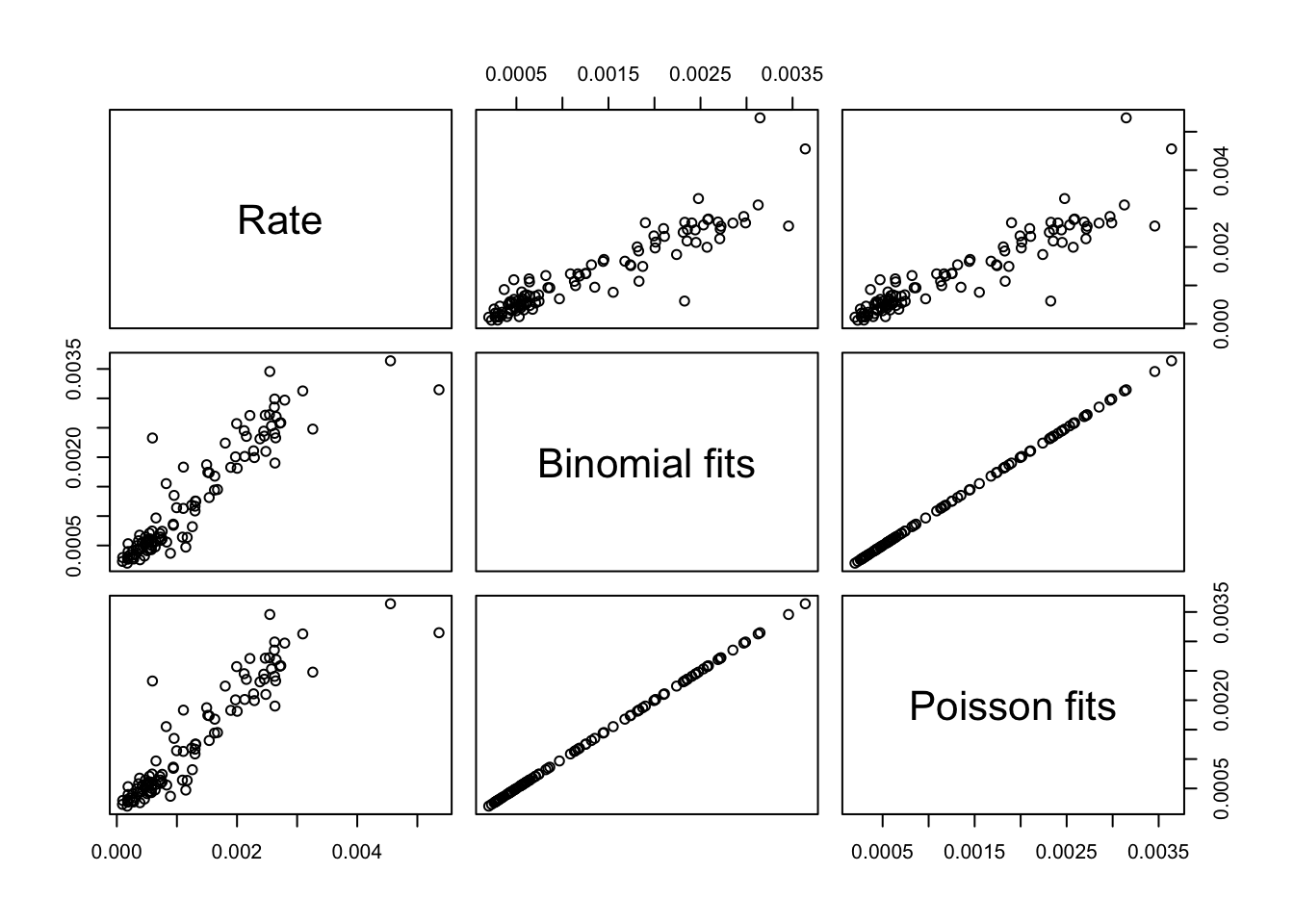
Methodologically, in modelling regional effects through indicators, we neglect the (most probably present) correlation between neighbouring regions. Moreover, through the indicators, one introduces a very large number of parameters, which eats up degrees of freedom, and so increases the variance of our estimators. There could also be a risk of separation and overfitting.
9.2.5 Dispersion and confidence interval for binomial GLM
For the rescaled binomial GLM, we have \(\mathcal{V}(\mu_i) = \mu_i (1 - \mu_i) / n_i\). Thus, we can estimate the dispersion for glm1 as follows.
V_bin <- glm1$fitted * (1 - glm1$fitted) / irlsuicide$pop
( phihat <- sum((irlsuicide$rate - glm1$fitted)^2 / V_bin) / glm1$df.res )
## [1] 2.990854To compute the confidence interval, we first implement the response function and then construct the interval as in the lecture notes.
h_func <- function(eta){
    exp(eta) / (1 + exp(eta))
}

eta_hat <- predict(glm3, newdata=data.frame(ID='3', age='3', sex='1'))
varhat <- summary(glm3)$cov.scaled # covariance matrix
x0 = c(1, 0, 1, 0, 1, 0, 1, 0, 0, 0, 0, 0, 0, 0, 0, 0, 0) # new data point
span <- qnorm(0.975) * sqrt( x0 %*%  varhat %*%  x0) # width of interval
c(h_func(eta_hat-span), h_func(eta_hat+span)) # confidence interval
## [1] 0.001694355 0.002960805Note that the way we construct x0 above is very clumsy and prone to errors. You should try to find a better way to do this.
9.3 Practical 3
Note that this solution uses the version of the data uploaded on Ultra, which contains the results of 270 games. If you use the latest data from the football website, your model may be different.
9.3.2 Fit and inspect the model
##
## Call:
## glm(formula = y ~ 0 + ., family = binomial(link = logit), data = matchdata)
##
## Coefficients:
##                 Estimate Std. Error z value Pr(>|z|)
## Aston.Villa      -1.2554     0.6008  -2.089 0.036676 *
## Bournemouth      -0.6303     0.6143  -1.026 0.304863
## Brentford        -1.2200     0.6149  -1.984 0.047266 *
## Brighton         -0.8547     0.6000  -1.425 0.154298
## Chelsea          -0.7203     0.6101  -1.181 0.237796
## Crystal.Palace   -1.2135     0.6089  -1.993 0.046255 *
## Everton          -1.3747     0.6112  -2.249 0.024501 *
## Fulham           -0.9204     0.6096  -1.510 0.131059
## Ipswich          -2.2148     0.6552  -3.381 0.000724 ***
## Leicester        -2.3562     0.6625  -3.556 0.000376 ***
## Liverpool         1.1120     0.7553   1.472 0.140950
## Man.City         -0.4222     0.6044  -0.699 0.484773
## Man.United       -1.0551     0.6138  -1.719 0.085634 .
## Newcastle        -0.6256     0.6143  -1.018 0.308496
## `Nott'm.Forest`  -0.5841     0.6021  -0.970 0.332072
## Southampton      -2.8853     0.7237  -3.987  6.7e-05 ***
## Tottenham        -1.5147     0.6101  -2.483 0.013037 *
## West.Ham         -1.1787     0.6038  -1.952 0.050923 .
## Wolves           -1.6646     0.6196  -2.687 0.007218 **
## ---
## Signif. codes:  0 '***' 0.001 '**' 0.01 '*' 0.05 '.' 0.1 ' ' 1
##
## (Dispersion parameter for binomial family taken to be 1)
##
##     Null deviance: 374.3  on 270  degrees of freedom
## Residual deviance: 308.0  on 251  degrees of freedom
## AIC: 346
##
## Number of Fisher Scoring iterations: 4## Liverpool Man.City `Nott'm.Forest` Newcastle Bournemouth
## 1.1119629 -0.4222423 -0.5840533 -0.6255966 -0.6302673
## Chelsea Brighton Fulham Man.United West.Ham
## -0.7202794 -0.8547381 -0.9204362 -1.0550582 -1.1786899
## Crystal.Palace Brentford Aston.Villa Everton Tottenham
## -1.2135390 -1.2199890 -1.2553757 -1.3746983 -1.5146809
## Wolves Ipswich Leicester Southampton
## -1.6645885 -2.2147949 -2.3561615 -2.8853025From the sorted coefficients, Man United seems much stronger than Tottenham compared to the league table. Notice that looking at the away games for these two teams, Man United achieved several draws which count as a “victory” when playing away under this model. Hence, the probability of away victories is likely inflated.
##           Date  Time       HomeTeam   AwayTeam FTHG FTAG
## 11  24/08/2024 12:30       Brighton Man United    2    1
## 31  14/09/2024 12:30    Southampton Man United    0    3
## 48  21/09/2024 17:30 Crystal Palace Man United    0    0
## 68  06/10/2024 14:00    Aston Villa Man United    0    0
## 89  27/10/2024 14:00       West Ham Man United    2    1
## 119 24/11/2024 16:30        Ipswich Man United    1    1
## 137 04/12/2024 20:15        Arsenal Man United    2    0
## 156 15/12/2024 16:30       Man City Man United    1    2
## 176 26/12/2024 17:30         Wolves Man United    2    0
## 198 05/01/2025 16:30      Liverpool Man United    2    2
## 229 26/01/2025 19:00         Fulham Man United    0    1
## 250 16/02/2025 16:30      Tottenham Man United    1    0
## 253 22/02/2025 12:30 Everton Man United 2 2## Date Time HomeTeam AwayTeam FTHG FTAG
## 10 19/08/2024 20:00 Leicester Tottenham 1 1
## 29 01/09/2024 13:30 Newcastle Tottenham 2 1
## 59 29/09/2024 16:30 Man United Tottenham 0 3
## 70 06/10/2024 16:30 Brighton Tottenham 3 2
## 88 27/10/2024 14:00 Crystal Palace Tottenham 1 0
## 117 23/11/2024 17:30 Man City Tottenham 0 4
## 140 05/12/2024 20:15 Bournemouth Tottenham 1 0
## 158 15/12/2024 19:00 Southampton Tottenham 0 5
## 174 26/12/2024 15:00 Nott'm Forest Tottenham 1 0
## 207 15/01/2025 20:00 Arsenal Tottenham 2 1
## 215 19/01/2025 14:00 Everton Tottenham 3 2
## 236 02/02/2025 14:00 Brentford Tottenham 0 2
## 257 22/02/2025 15:00 Ipswich Tottenham 1 49.3.3 Model home team advantage
A home team advantage could be modelled as a constant multiplicative effect on the odds of a home team win. This is exactly the effect an intercept term would have. So, we can drop the 0+ in the model formula to allow for an intercept:
##
## Call:
## glm(formula = y ~ ., family = binomial(link = logit), data = matchdata)
##
## Coefficients:
##                 Estimate Std. Error z value Pr(>|z|)
## (Intercept)      -0.5228     0.1441  -3.629 0.000285 ***
## Aston.Villa      -1.2310     0.6155  -2.000 0.045487 *
## Bournemouth      -0.6116     0.6365  -0.961 0.336587
## Brentford        -1.2161     0.6337  -1.919 0.054976 .
## Brighton         -0.8474     0.6142  -1.380 0.167699
## Chelsea          -0.6873     0.6330  -1.086 0.277582
## Crystal.Palace   -1.2178     0.6300  -1.933 0.053252 .
## Everton          -1.3647     0.6274  -2.175 0.029615 *
## Fulham           -0.8880     0.6274  -1.415 0.156998
## Ipswich          -2.2457     0.6676  -3.364 0.000769 ***
## Leicester        -2.3909     0.6866  -3.482 0.000497 ***
## Liverpool         1.1908     0.7751   1.536 0.124490
## Man.City         -0.4048     0.6218  -0.651 0.514987
## Man.United       -1.0270     0.6274  -1.637 0.101638
## Newcastle        -0.6231     0.6348  -0.982 0.326309
## `Nott'm.Forest`  -0.5848     0.6168  -0.948 0.343027
## Southampton      -2.9704     0.7350  -4.042 5.31e-05 ***
## Tottenham        -1.5179     0.6253  -2.427 0.015205 *
## West.Ham         -1.1822     0.6198  -1.908 0.056455 .
## Wolves           -1.7324     0.6365  -2.722 0.006491 **
## ---
## Signif. codes:  0 '***' 0.001 '**' 0.01 '*' 0.05 '.' 0.1 ' ' 1
##
## (Dispersion parameter for binomial family taken to be 1)
##
##     Null deviance: 361.74  on 269  degrees of freedom
## Residual deviance: 294.24  on 250  degrees of freedom
## AIC: 334.24
##
## Number of Fisher Scoring iterations: 5
The intercept is actually negative! Looking at the standard error for the intercept, the actual coefficient value is negative with high probability. Thus, home teams are at a disadvantage according to the model.
9.3.4 Estimate the dispersion
We expect a logistic regression to have theoretical dispersion parameter 1. We can obtain a quick estimate of the actual dispersion:
## [1] 1.227091## [1] 1.176971The dispersion reduced when adding the intercept into the model. There is overdispersion in both models, but possibly not very bad.
9.3.5 Prediction and hypothesis testing
To prepare the data for the new match, it is easiest to pull a row from X, zero out and then set the home/away teams we need:
##   Aston.Villa Bournemouth Brentford Brighton Chelsea Crystal.Palace Everton
## 1           0           0         0        1       0              0       0
##   Fulham Ipswich Leicester Liverpool Man.City Man.United Newcastle
## 1     -1       0         0         0        0          0         0
##   Nott'm.Forest Southampton Tottenham West.Ham Wolves
## 1             0           0         0        0      0
The probability of a draw or win for Fulham is the probability of away win according to our model, which is:
##       1
## 0.61826
To perform the hypothesis test, we need to fit the model with the three teams fixed to the same coefficient. To do this, simply tell R to remove the individual predictors and insert a new predictor formed from all three.
fit3 <- glm(y ~ . - Ipswich - Leicester - Southampton
                + I(Ipswich + Leicester + Southampton),
            matchdata, family = binomial(link=logit))
summary(fit3)
##
## Call:
## glm(formula = y ~ . - Ipswich - Leicester - Southampton + I(Ipswich +
## Leicester + Southampton), family = binomial(link = logit),
## data = matchdata)
##
## Coefficients:
## Estimate Std. Error z value Pr(>|z|)
## (Intercept) -0.5191 0.1438 -3.609 0.000307 ***
## Aston.Villa -1.2364 0.6159 -2.007 0.044706 *
## Bournemouth -0.5966 0.6351 -0.939 0.347537
## Brentford -1.2087 0.6326 -1.911 0.056067 .
## Brighton -0.8406 0.6135 -1.370 0.170653
## Chelsea -0.6728 0.6317 -1.065 0.286853
## Crystal.Palace -1.2131 0.6297 -1.926 0.054061 .
## Everton -1.3677 0.6274 -2.180 0.029269 *
## Fulham -0.8916 0.6278 -1.420 0.155533
## Liverpool 1.1888 0.7753 1.533 0.125199
## Man.City -0.4044 0.6217 -0.651 0.515336
## Man.United -1.0239 0.6269 -1.633 0.102402
## Newcastle -0.6113 0.6337 -0.965 0.334726
## `Nott'm.Forest` -0.5751 0.6158 -0.934 0.350359
## Tottenham -1.5321 0.6260 -2.448 0.014381 *
## West.Ham -1.1841 0.6196 -1.911 0.055996 .
## Wolves -1.7245 0.6358 -2.712 0.006679 **
## I(Ipswich + Leicester + Southampton) -2.5113 0.5619 -4.469 7.85e-06 ***
## ---
## Signif. codes: 0 '***' 0.001 '**' 0.01 '*' 0.05 '.' 0.1 ' ' 1
##
## (Dispersion parameter for binomial family taken to be 1)
##
## Null deviance: 361.74 on 269 degrees of freedom
## Residual deviance: 295.44 on 252 degrees of freedom
## AIC: 331.44
##
## Number of Fisher Scoring iterations: 5In logistic regression, the dispersion is 1, so the likelihood ratio test statistic can be found by just taking the difference of the deviances:
## [1] 1.198313The difference in degrees of freedom is (should be 2 as we have replaced 3 coefficients with 1):
## [1] 2The test is against \(\chi^2(2)\):
## [1] 5.991465The likelihood ratio statistic is not larger, therefore we do not have enough evidence to reject the reduced model. Plausibly, all teams up for relegation are equally weak.
9.3.6 Plot the confidence region
We get the full Fisher information matrix and extract the submatrix involving Leicester and Man City. Then we inverse this submatrix to obtain \(F(\hat{\boldsymbol\beta})\).
##           Leicester  Man.City
## Leicester  2.737449 -1.434316
## Man.City  -1.434316  3.337963
The MLEs for these two teams are:
We define the mahalanobis2 function:
mahalanobis2 <- function(beta_l, beta_mc) {
                  beta <- c(beta_l, beta_mc)
                  t(betahat_lmc - beta) %*% F_lmc %*% (betahat_lmc - beta)
                }
and setup the grid:
We evaluate the distance over the grid:
We colour the confidence region and mark the location of the MLEs. Optionally, you can also add the individual confidence intervals calculated by R as horizontal and vertical lines. However, note that the confint function below is doing something called profiling to get the intervals that account for all other variables, so you will notice a small discrepancy between the marginal intervals and the plotted region.
image(leicester, man_city, HessCR <= qchisq(0.95, 2))
points(betahat_lmc[1], betahat_lmc[2], pch = 3, col = "green")

abline(h = confint(fit2, "Man.City"))
abline(v = confint(fit2, "Leicester"))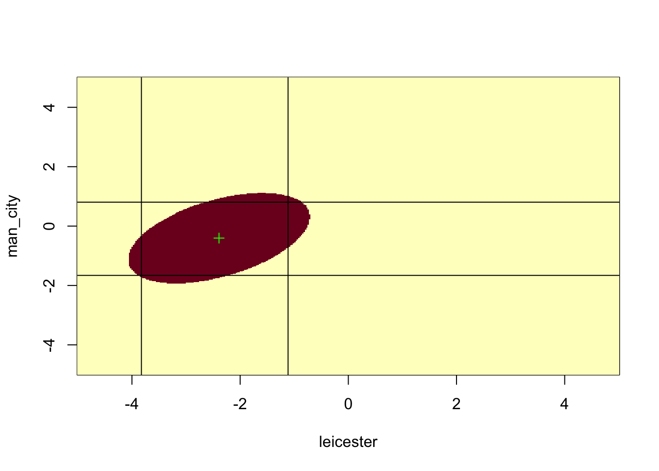
9.4 Practical 4
9.4.1 Part 1: Pupil extraversion data
9.4.1.2 Exploratory analysis
We plot the popularity variable:
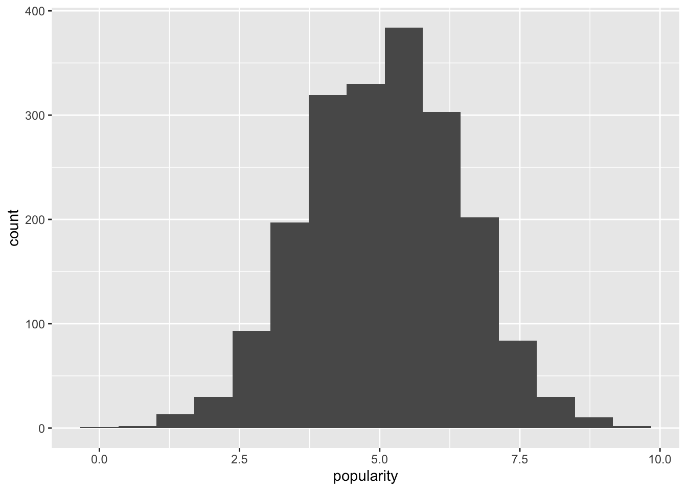
This plot indicates that a Gaussian response distribution appears to be a reasonable assumption.
Next let’s look at the three predictor variables.
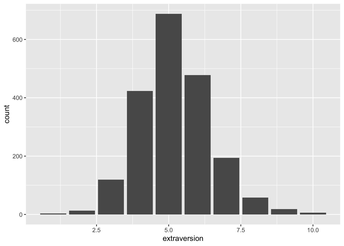
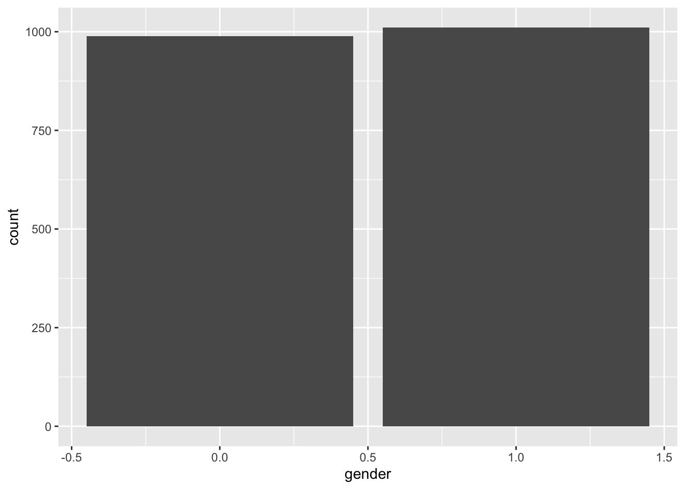
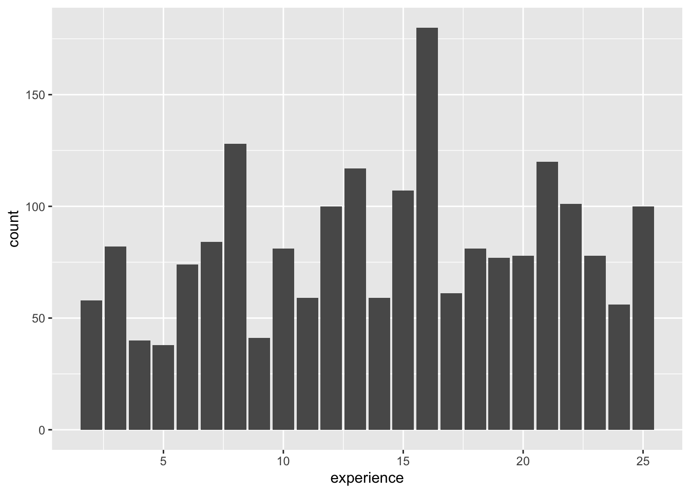
The shape of the distribution of predictor variables is not of importance from a statistical modelling point of view.
We plot popularity versus extraversion and add a simple linear regression line:
ggplot(data=pop.data, aes(x=extraversion, y=popularity)) +
    geom_point(size=1, alpha=.8) +
    geom_smooth(method="lm", col="red", linewidth=1, alpha=.8, se=FALSE)
## `geom_smooth()` using formula = 'y ~ x'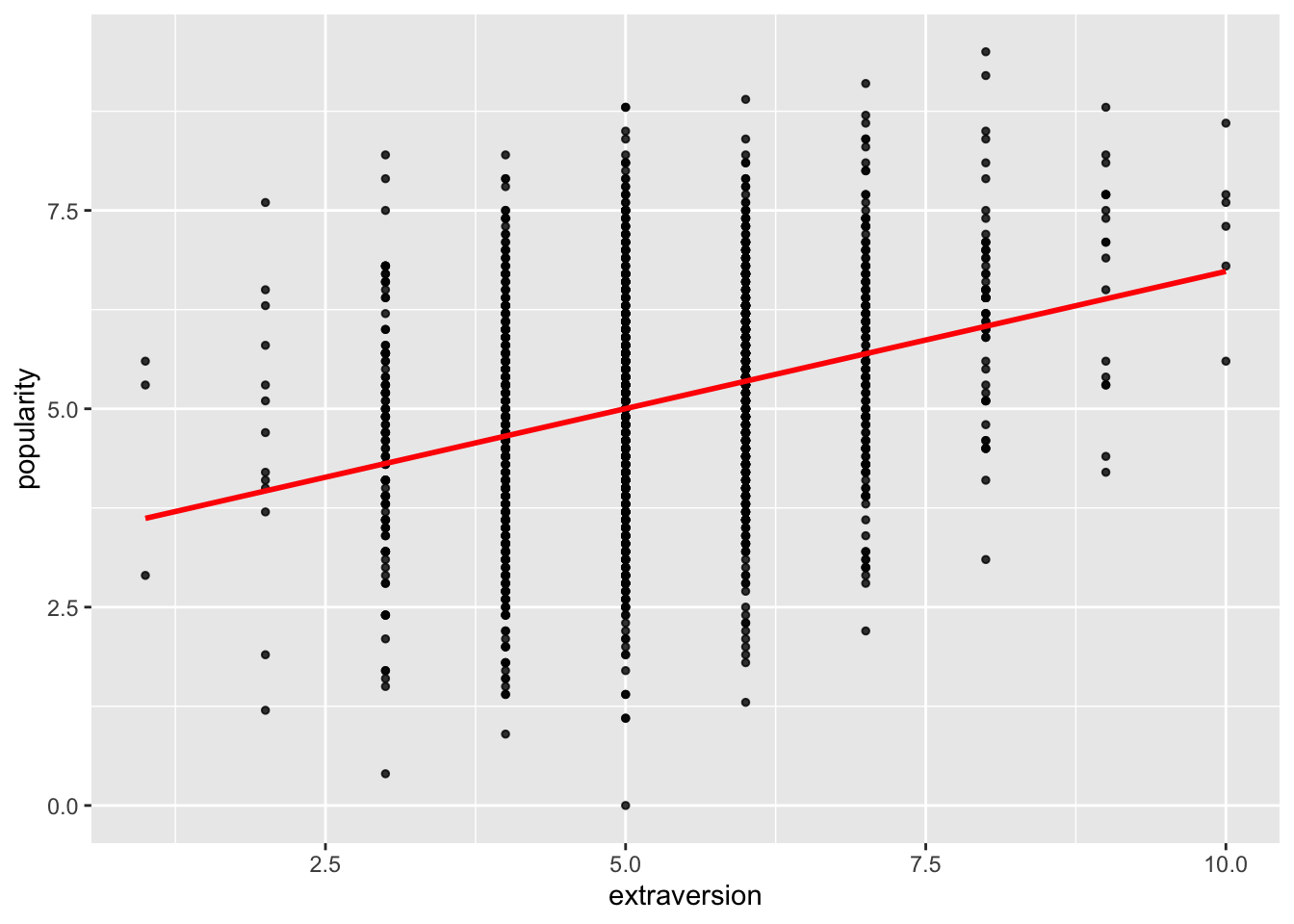
We plot a scatter plot of popularity versus extraversion coloured by class, and then add class-specific linear regression lines:
ggplot(data=pop.data,
       aes(x=extraversion, y=popularity, colour=as.factor(class))) +
    geom_jitter(size=0.8) +  # to add some random noise for plotting purposes
    labs(title="Popularity versus extraversion", subtitle="by class") +
    theme(legend.position="none") +
    geom_smooth(method="lm", se=FALSE)
## `geom_smooth()` using formula = 'y ~ x'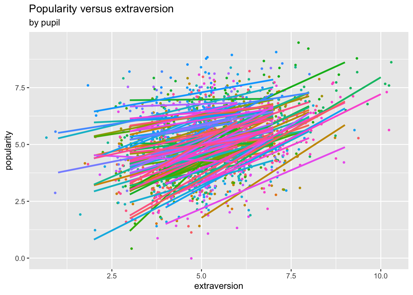
9.4.1.3 Modelling
We fit and compare the simple linear model as well as the three marginal models.
##
## Call:
## lm(formula = popularity ~ extraversion, data = pop.data)
##
## Residuals:
##     Min      1Q  Median      3Q     Max
## -5.0021 -0.9021  0.0062  0.8896  3.8896
##
## Coefficients:
##              Estimate Std. Error t value Pr(>|t|)
## (Intercept)   3.27284    0.12474   26.24   <2e-16 ***
## extraversion  0.34585    0.02325   14.88   <2e-16 ***
## ---
## Signif. codes:  0 '***' 0.001 '**' 0.01 '*' 0.05 '.' 0.1 ' ' 1
##
## Residual standard error: 1.312 on 1998 degrees of freedom
## Multiple R-squared:  0.09973,    Adjusted R-squared:  0.09927
## F-statistic: 221.3 on 1 and 1998 DF, p-value: < 2.2e-16## Beginning Cgee S-function, @(#) geeformula.q 4.13 98/01/27## running glm to get initial regression estimate## (Intercept) extraversion
## 3.2728356 0.3458513##
## GEE: GENERALIZED LINEAR MODELS FOR DEPENDENT DATA
## gee S-function, version 4.13 modified 98/01/27 (1998)
##
## Model:
## Link: Identity
## Variance to Mean Relation: Gaussian
## Correlation Structure: Independent
##
## Call:
## gee(formula = popularity ~ extraversion, id = pop.data$class,
## data = pop.data, corstr = "independence")
##
## Number of observations : 2000
##
## Maximum cluster size : 26
##
##
## Coefficients:
##  (Intercept) extraversion
##    3.2728356    0.3458513
##
## Estimated Scale Parameter: 1.721615
## Number of Iterations: 1
##
## Working Correlation[1:4,1:4]
## [,1] [,2] [,3] [,4]
## [1,] 1 0 0 0
## [2,] 0 1 0 0
## [3,] 0 0 1 0
## [4,] 0 0 0 1
##
##
## Returned Error Value:
## [1] 0## Estimate Naive S.E. Naive z Robust S.E. Robust z
## (Intercept) 3.2728356 0.12473523 26.23826 0.24462310 13.379095
## extraversion 0.3458513 0.02324748 14.87694 0.04024471 8.593708Clearly this model is just equivalent to the simple linear model (including the standard errors!). Note also that \(1.312^2=1.721\).
## Beginning Cgee S-function, @(#) geeformula.q 4.13 98/01/27## running glm to get initial regression estimate## (Intercept) extraversion
## 3.2728356 0.3458513##
## GEE: GENERALIZED LINEAR MODELS FOR DEPENDENT DATA
## gee S-function, version 4.13 modified 98/01/27 (1998)
##
## Model:
## Link: Identity
## Variance to Mean Relation: Gaussian
## Correlation Structure: Exchangeable
##
## Call:
## gee(formula = popularity ~ extraversion, id = pop.data$class,
## data = pop.data, corstr = "exchangeable")
##
## Number of observations : 2000
##
## Maximum cluster size : 26
##
##
## Coefficients:
## (Intercept) extraversion
## 2.5453601 0.4856898
##
## Estimated Scale Parameter: 1.752796
## Number of Iterations: 3
##
## Working Correlation[1:4,1:4]
## [,1] [,2] [,3] [,4]
## [1,] 1.0000000 0.4602074 0.4602074 0.4602074
## [2,] 0.4602074 1.0000000 0.4602074 0.4602074
## [3,] 0.4602074 0.4602074 1.0000000 0.4602074
## [4,] 0.4602074 0.4602074 0.4602074 1.0000000
##
##
## Returned Error Value:
## [1] 0## Estimate Naive S.E. Naive z Robust S.E. Robust z
## (Intercept) 2.5453601 0.14057079 18.10732 0.20630224 12.33801
## extraversion 0.4856898 0.02031064 23.91308 0.02654914 18.29399The parameter estimates appear to have changed quite a lot after providing the correlation structure. Standard errors have changed slightly.
## Beginning Cgee S-function, @(#) geeformula.q 4.13 98/01/27## running glm to get initial regression estimate## (Intercept) extraversion
## 3.2728356 0.3458513##
## GEE: GENERALIZED LINEAR MODELS FOR DEPENDENT DATA
## gee S-function, version 4.13 modified 98/01/27 (1998)
##
## Model:
## Link: Identity
## Variance to Mean Relation: Gaussian
## Correlation Structure: Unstructured
##
## Call:
## gee(formula = popularity ~ extraversion, id = pop.data$class,
## data = pop.data, corstr = "unstructured")
##
## Number of observations : 2000
##
## Maximum cluster size : 26
##
##
## Coefficients:
## (Intercept) extraversion
## 2.5929361 0.4850722
##
## Estimated Scale Parameter: 1.754649
## Number of Iterations: 5
##
## Working Correlation[1:4,1:4]
## [,1] [,2] [,3] [,4]
## [1,] 1.0000000 0.3810784 0.3487750 0.5073841
## [2,] 0.3810784 1.0000000 0.3178906 0.7057648
## [3,] 0.3487750 0.3178906 1.0000000 0.4382877
## [4,] 0.5073841 0.7057648 0.4382877 1.0000000
##
##
## Returned Error Value:
## [1] 0## Estimate Naive S.E. Naive z Robust S.E. Robust z
## (Intercept) 2.5929361 0.11672601 22.21387 0.16444742 15.76757
## extraversion 0.4850722 0.01759611 27.56702 0.02039971 23.77838The two models using exchangeable and unstructured correlation matrices give very similar parameter estimates. The standard errors of the latter model appear to be a bit smaller, and the differences in the entries of its estimated correlation matrix appear to be quite large (i.e., quite different from the exchangeable correlation structure assumption). So, perhaps this is the one to use.
We now add the estimated regression lines from the exchangeable and unstructured models to the original scatter plot with the least squares fit.
pred1  <- predict(pop.gee1)
frame1 <- unique(data.frame(extraversion=pop.data$extraversion, pred1=pred1))

pred2 <- predict(pop.gee2)
frame2<- unique(data.frame(extraversion=pop.data$extraversion, pred2=pred2))

ggplot(data = pop.data, aes(x=extraversion, y=popularity)) +
    geom_point(size = 1, alpha = .8) +
    geom_smooth(method = "lm", # to add regression line
                col = "red", linewidth = 1, alpha = .8, se = FALSE) +
    geom_line(data=frame1, aes(x=extraversion, y=pred1), col="Blue") +
    geom_line(data=frame2, aes(x=extraversion, y=pred2), col="Green")
## `geom_smooth()` using formula = 'y ~ x'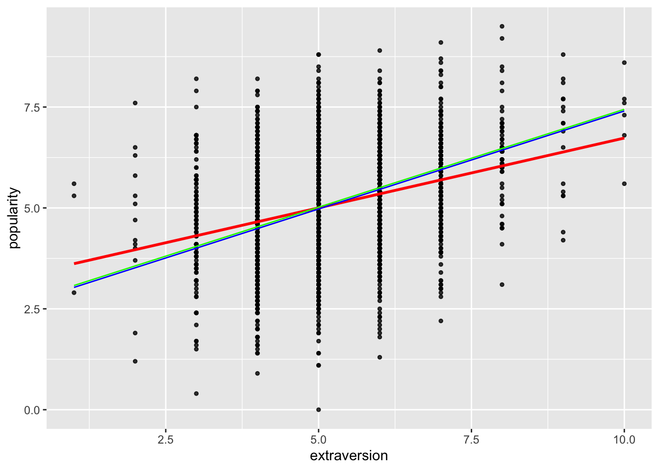
Easier (but not as nice) without ggplot:
plot(pop.data$extraversion, pop.data$popularity)
abline(pop.simple)
lines(pop.data$extraversion, pred1, col=2)
lines(pop.data$extraversion, pred2, col=3)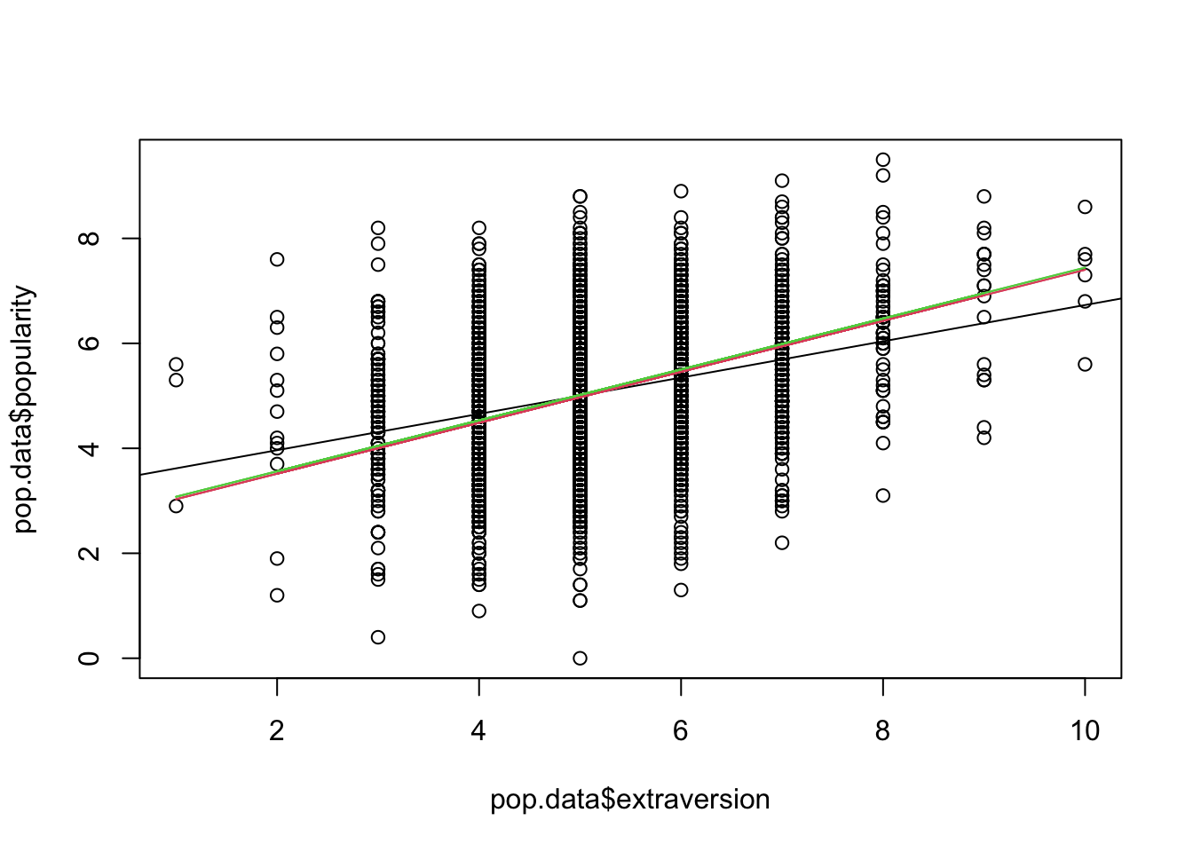
The fitted marginal models appear to identify a stronger effect (slope) as compared to the linear model fit. (This is a potentially important finding!)
Finally, we fit the GEE models under the three variance specifications, but now including the additional covariates gender and experience.
pop.gee0a <- gee(popularity~extraversion+gender+experience, id=pop.data$class,
                 corstr="independence", data=pop.data)
## Beginning Cgee S-function, @(#) geeformula.q 4.13 98/01/27## running glm to get initial regression estimate## (Intercept) extraversion gender experience
## 0.63230670 0.47543435 1.37926173 0.08886885##
## GEE: GENERALIZED LINEAR MODELS FOR DEPENDENT DATA
## gee S-function, version 4.13 modified 98/01/27 (1998)
##
## Model:
## Link: Identity
## Variance to Mean Relation: Gaussian
## Correlation Structure: Independent
##
## Call:
## gee(formula = popularity ~ extraversion + gender + experience,
## id = pop.data$class, data = pop.data, corstr = "independence")
##
## Number of observations : 2000
##
## Maximum cluster size : 26
##
##
## Coefficients:
##  (Intercept) extraversion       gender   experience
##   0.63230670   0.47543435   1.37926173   0.08886885
##
## Estimated Scale Parameter: 0.8756509
## Number of Iterations: 1
##
## Working Correlation[1:4,1:4]
## [,1] [,2] [,3] [,4]
## [1,] 1 0 0 0
## [2,] 0 1 0 0
## [3,] 0 0 1 0
## [4,] 0 0 0 1
##
##
## Returned Error Value:
## [1] 0## Estimate Naive S.E. Naive z Robust S.E. Robust z
## (Intercept) 0.63230670 0.123545138 5.118022 0.208810204 3.028141
## extraversion 0.47543435 0.018126163 26.229177 0.028922707 16.438100
## gender 1.37926173 0.042307923 32.600554 0.065013144 21.215121
## experience 0.08886885 0.003487737 25.480377 0.008556324 10.386335pop.gee1a <- gee(popularity~extraversion+gender+experience, id=pop.data$class,
corstr="exchangeable", data=pop.data)## Beginning Cgee S-function, @(#) geeformula.q 4.13 98/01/27
## running glm to get initial regression estimate## (Intercept) extraversion gender experience
## 0.63230670 0.47543435 1.37926173 0.08886885##
## GEE: GENERALIZED LINEAR MODELS FOR DEPENDENT DATA
## gee S-function, version 4.13 modified 98/01/27 (1998)
##
## Model:
## Link: Identity
## Variance to Mean Relation: Gaussian
## Correlation Structure: Exchangeable
##
## Call:
## gee(formula = popularity ~ extraversion + gender + experience,
## id = pop.data$class, data = pop.data, corstr = "exchangeable")
##
## Number of observations : 2000
##
## Maximum cluster size : 26
##
##
## Coefficients:
## (Intercept) extraversion gender experience
## 0.80885713 0.45454004 1.25440929 0.08841021
##
## Estimated Scale Parameter: 0.8805257
## Number of Iterations: 3
##
## Working Correlation[1:4,1:4]
## [,1] [,2] [,3] [,4]
## [1,] 1.0000000 0.3231302 0.3231302 0.3231302
## [2,] 0.3231302 1.0000000 0.3231302 0.3231302
## [3,] 0.3231302 0.3231302 1.0000000 0.3231302
## [4,] 0.3231302 0.3231302 0.3231302 1.0000000
##
##
## Returned Error Value:
## [1] 0## Estimate Naive S.E. Naive z Robust S.E. Robust z
## (Intercept) 0.80885713 0.16837377 4.803938 0.206419039 3.918520
## extraversion 0.45454004 0.01621439 28.033120 0.024598838 18.478110
## gender 1.25440929 0.03740518 33.535706 0.036410480 34.451875
## experience 0.08841021 0.00862302 10.252813 0.008984785 9.839991pop.gee2a <- gee(popularity~extraversion+gender+experience, id=pop.data$class,
corstr="unstructured", data=pop.data)## Beginning Cgee S-function, @(#) geeformula.q 4.13 98/01/27
## running glm to get initial regression estimate## (Intercept) extraversion gender experience
## 0.63230670 0.47543435 1.37926173 0.08886885##
## GEE: GENERALIZED LINEAR MODELS FOR DEPENDENT DATA
## gee S-function, version 4.13 modified 98/01/27 (1998)
##
## Model:
## Link: Identity
## Variance to Mean Relation: Gaussian
## Correlation Structure: Unstructured
##
## Call:
## gee(formula = popularity ~ extraversion + gender + experience,
## id = pop.data$class, data = pop.data, corstr = "unstructured")
##
## Number of observations : 2000
##
## Maximum cluster size : 26
##
##
## Coefficients:
## (Intercept) extraversion gender experience
## 0.82549133 0.45787157 1.25396183 0.08678284
##
## Estimated Scale Parameter: 0.8804735
## Number of Iterations: 4
##
## Working Correlation[1:4,1:4]
## [,1] [,2] [,3] [,4]
## [1,] 1.0000000 0.2847368 0.2604985 0.3783846
## [2,] 0.2847368 1.0000000 0.1683386 0.6066850
## [3,] 0.2604985 0.1683386 1.0000000 0.3209093
## [4,] 0.3783846 0.6066850 0.3209093 1.0000000
##
##
## Returned Error Value:
## [1] 0## Estimate Naive S.E. Naive z Robust S.E. Robust z
## (Intercept) 0.82549133 0.144312100 5.720181 0.182576163 4.521353
## extraversion 0.45787157 0.014391955 31.814411 0.020383817 22.462504
## gender 1.25396183 0.033715675 37.192250 0.035116333 35.708792
## experience 0.08678284 0.007362563 11.787042 0.008104102 10.708508Again the last two variance specifications yield very similar parameter estimates, with smaller standard errors for the unstructured one.
9.4.2 Part 2: Childweight data
We fit the random intercept model:
We extract and visualize the fitted values of this random intercept model as well as the linear model fits:
childweight$pred1 <- predict(lmm1)

ggplot(childweight, aes(age, weight)) +
    geom_line(aes(y=pred1, col=id)) +
    geom_point(aes(age, weight, col=id)) +
    geom_smooth(method="lm", se=FALSE, col="Red") +
    ggtitle("Model lmm1", subtitle="random intercept-only") +
    xlab("age") +
    ylab("weight") +
    theme(legend.position="none")
## `geom_smooth()` using formula = 'y ~ x'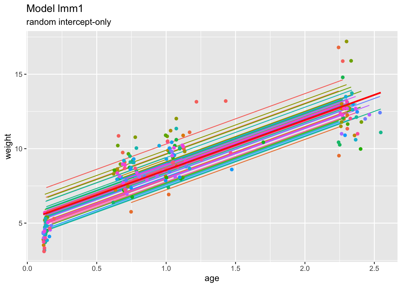
Clearly, under this model, the predicted trends for the individuals are just vertical translations of the overall (marginal) trend.
We expand the previous model by including a random slope for age:
## Linear mixed model fit by REML. t-tests use Satterthwaite's method [
## lmerModLmerTest]
## Formula: weight ~ age + girl + (age | id)
##    Data: childweight
##
## REML criterion at convergence: 684.1
##
## Scaled residuals:
##      Min       1Q   Median       3Q      Max
## -2.38416 -0.69583 -0.04232  0.73479  2.13691
##
## Random effects:
##  Groups   Name        Variance Std.Dev. Corr
##  id       (Intercept) 0.05702  0.2388
##           age         0.20709  0.4551   1.00
##  Residual             1.36994  1.1704
## Number of obs: 198, groups:  id, 68
##
## Fixed effects:
##             Estimate Std. Error       df t value Pr(>|t|)
## (Intercept)   5.4293     0.1869 121.3239  29.051  < 2e-16 ***
## age           3.4593     0.1264  70.9320  27.362  < 2e-16 ***
## girl         -0.6354     0.2316  71.3148  -2.744  0.00767 **
## ---
## Signif. codes:  0 '***' 0.001 '**' 0.01 '*' 0.05 '.' 0.1 ' ' 1
##
## Correlation of Fixed Effects:
##      (Intr) age
## age  -0.488
## girl -0.612 -0.006
We visualize the fitted values of this model:
childweight$pred2 <- predict(lmm2)

ggplot(childweight, aes(age, weight)) +
    geom_line(aes(y=pred2, col=id)) +
    geom_point(aes(age, weight, col=id)) +
    geom_smooth(method="lm", se=FALSE, col="Red") +
    ggtitle("Model lmm2", subtitle="random intercept and slope") +
    xlab("Age (Time)") +
    ylab("Weight") +
    theme(legend.position="none")
## `geom_smooth()` using formula = 'y ~ x'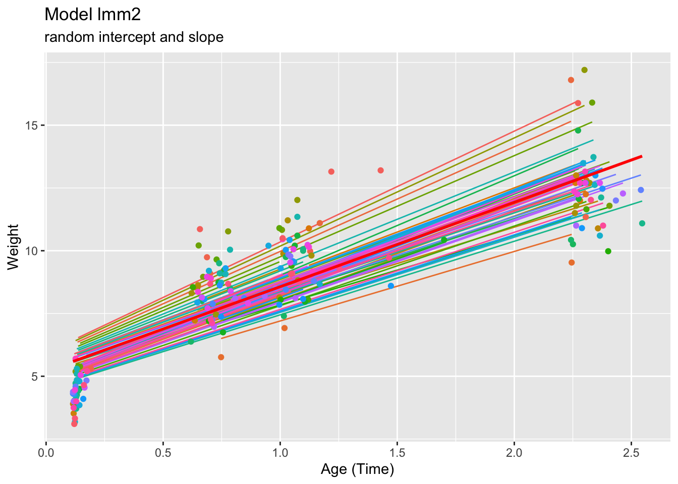
We extract and inspect the variance-covariance matrix:
##  Groups   Name        Std.Dev. Corr
##  id       (Intercept) 0.23879
##           age         0.45507  1.000
##  Residual             1.17045
The positive covariance re-affirms the fanning out pattern observed. The higher the predicted weight at baseline time (higher child intercept), the higher the weight will be as time passes (steeper intercept slope).
The correlation value appears noteworthy – we consider therefore the random effects in more detail.
## $id
##       (Intercept)          age
## 45    0.501946747  0.956593268
## 258   0.029304921  0.055848318
## 287   0.373042397  0.710931698
## 483  -0.361818464 -0.689541489
## 725  -0.069448256 -0.132352152
## 800   0.032523923  0.061982996
## 801  -0.173762135 -0.331150036
## 832  -0.024082103 -0.045894854
## 833  -0.042949990 -0.081852645
## 944  -0.292523234 -0.557480962
## 1005  0.130570836  0.248837514
## 1010 -0.011479161 -0.021876614
## 1055  0.074717224  0.142393573
## 1141 -0.070778563 -0.134887407
## 1155  0.446035652  0.850039790
## 1249  0.217952283  0.415366140
## 1264 -0.038049114 -0.072512743
## 1291  0.299154085  0.570117820
## 1341  0.233975253  0.445902184
## 1417 -0.151307222 -0.288356221
## 1441  0.035264989  0.067206839
## 1572 -0.360593828 -0.687207628
## 1614 -0.081002898 -0.154372604
## 1976 -0.001865144 -0.003554527
## 2088  0.112817409  0.215003619
## 2106  0.264568952  0.504206632
## 2108 -0.221943115 -0.422971744
## 2130 -0.230919595 -0.440078819
## 2150  0.135401386  0.258043423
## 2197  0.106174225  0.202343281
## 2251 -0.277556179 -0.528957251
## 2302 -0.174226938 -0.332035850
## 2317  0.091710846  0.174779455
## 2351  0.164092467  0.312721914
## 2353  0.001049086  0.001999313
## 2433  0.064315264  0.122569867
## 2615 -0.243616997 -0.464277093
## 2661  0.135404092  0.258048574
## 2730  0.045838082  0.087356689
## 2817 -0.083516516 -0.159162971
## 2850  0.150867155  0.287517550
## 3021  0.012182015  0.023216070
## 3148 -0.224594633 -0.428024913
## 3171 -0.040690223 -0.077546061
## 3192  0.049757490  0.094826146
## 3289 -0.087099484 -0.165991265
## 3446 -0.205747177 -0.392106063
## 3556 -0.143285330 -0.273068376
## 3672  0.016210964  0.030894313
## 3714  0.028683032  0.054663160
## 3827 -0.097672942 -0.186141818
## 3860 -0.108771374 -0.207292836
## 4017 -0.073815422 -0.140674945
## 4081  0.081215574  0.154777912
## 4108 -0.042719992 -0.081414332
## 4119  0.029366238  0.055965192
## 4139  0.120645683  0.229922486
## 4152  0.065761661  0.125326362
## 4169  0.269695037  0.513975745
## 4357 -0.084631204 -0.161287311
## 4418 -0.064870541 -0.123628101
## 4475  0.010313103  0.019654376
## 4518 -0.066985332 -0.127658389
## 4666 -0.203246594 -0.387340543
## 4682 -0.161260541 -0.307324929
## 4826  0.160832970  0.306510078
## 4841 -0.010735024 -0.020458437
## 4975  0.036174220  0.068939629
##
## with conditional variances for "id"## $id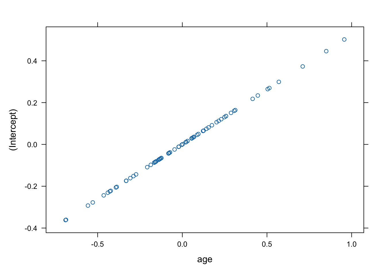
Indeed this is rather unusual – the correlation between the two random effects is equal to 1, and so the random intercept determines the random slope.
9.4.2.1 Diagnostics and model comparison
We inspect the residuals of the random slope model:
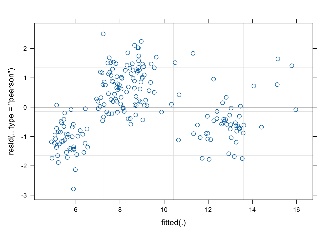
We include a quadratic term for age and produce again the residual plot:
## Linear mixed model fit by REML. t-tests use Satterthwaite's method [
## lmerModLmerTest]
## Formula: weight ~ age + c(age^2) + girl + (age | id)
##    Data: childweight
##
## REML criterion at convergence: 518
##
## Scaled residuals:
##      Min       1Q   Median       3Q      Max
## -2.04189 -0.44260 -0.03241  0.41940  2.66968
##
## Random effects:
##  Groups   Name        Variance Std.Dev. Corr
##  id       (Intercept) 0.3781   0.6149
##           age         0.2681   0.5178   0.14
##  Residual             0.3296   0.5741
## Number of obs: 198, groups:  id, 68
##
## Fixed effects:
##              Estimate Std. Error        df t value Pr(>|t|)
## (Intercept)   3.79550    0.16815  85.13224  22.573  < 2e-16 ***
## age           7.69844    0.23985 130.74444  32.096  < 2e-16 ***
## c(age^2)     -1.65773    0.08859 111.71023 -18.711  < 2e-16 ***
## girl         -0.59838    0.19997  57.23067  -2.992  0.00408 **
## ---
## Signif. codes:  0 '***' 0.001 '**' 0.01 '*' 0.05 '.' 0.1 ' ' 1
##
## Correlation of Fixed Effects:
##          (Intr) age    c(g^2)
## age      -0.543
## c(age^2)  0.502 -0.929
## girl     -0.588 -0.008  0.007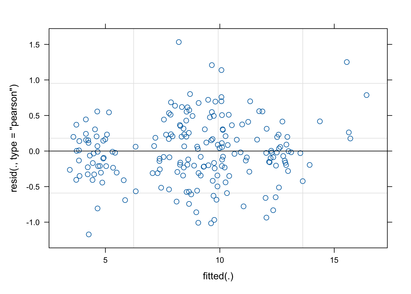
It is evident that the non-linearity has been controlled for and residuals look much more acceptable.
Assess the significance of the quadratic term:
##      Estimate    Std. Error            df       t value      Pr(>|t|)
## -1.657734e+00 8.859459e-02 1.117102e+02 -1.871146e+01 3.216673e-36## refitting model(s) with ML (instead of REML)## Data: childweight
## Models:
## lmm2: weight ~ age + girl + (age | id)
## lmm3: weight ~ age + c(age^2) + girl + (age | id)
## npar AIC BIC logLik deviance Chisq Df Pr(>Chisq)
## lmm2 7 692.20 715.22 -339.10 678.20
## lmm3 8 523.73 550.04 -253.87 507.73 170.47 1 < 2.2e-16 ***
## ---
## Signif. codes: 0 '***' 0.001 '**' 0.01 '*' 0.05 '.' 0.1 ' ' 1## Computing profile confidence intervals ...## 2.5 % 97.5 %
## .sig01 0.3021246 0.8504830
## .sig02 -0.3333909 1.0000000
## .sig03 0.3391380 0.6956586
## .sigma 0.4865445 0.6835441
## (Intercept) 3.4645810 4.1273140
## age 7.2255932 8.1697487
## c(age^2) -1.8333875 -1.4832757
## girl -0.9986598 -0.1996319Firstly, we observe from the fitted model summary that the absolute t-value for the squared age coefficient is approximately \(18 \gg 2\). Then, we see that the LR test gives a chi-square statistic of \(170.47\) at 1df, which is higher than any reasonable quantile of that distribution. Finally, the \(95\%\) confidence interval for c(age^2) clearly does not contain \(0\). Thus, there is very strong evidence to include the quadratic term.
We check the QQ plots of residuals:
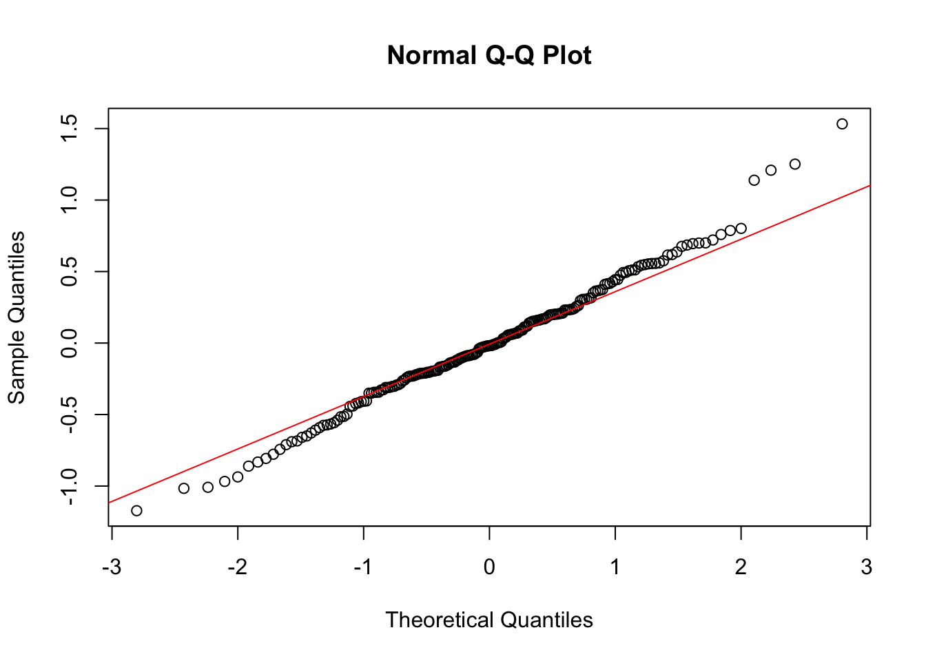
There might be some violation; the tails appear to be a bit thicker than they should be.
Now we check the random effects:
par(mfrow=c(1,2))
qqnorm(ranef(lmm3)$id[,1])
qqline(ranef(lmm3)$id[,1], col="red")
qqnorm(ranef(lmm3)$id[,2])
qqline(ranef(lmm3)$id[,2], col="red")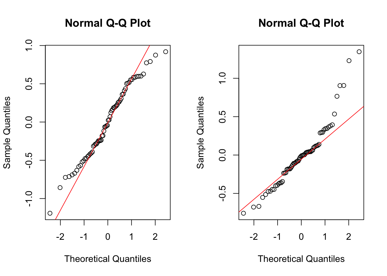
This does not look great, but on the other hand, the normality of the random effects is rather a technical assumption than a modelling assumption. Hence, less perfection of adherence to this assumption is expected as compared to the residual plot.
Finally, we again look at the fitted curves of this model:
childweight$pred3 <- predict(lmm3)

ggplot(childweight, aes(age,weight)) +
    geom_line(aes(y=pred3, col=id)) +
    geom_point(aes(age, weight, col=id)) +
    geom_smooth(method="lm", se=FALSE, col="Red") +
    ggtitle("Model lmm3", subtitle="random intercept and slope") +
    xlab("age") +
    ylab("weight") +
    theme(legend.position="none")
## `geom_smooth()` using formula = 'y ~ x'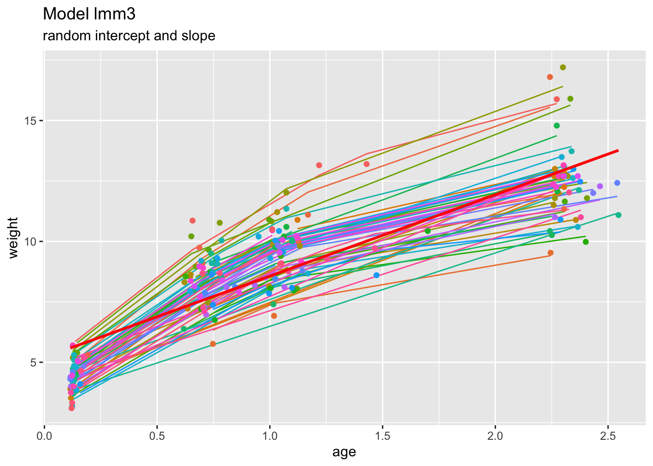
This appears a more realistic description of the data, capturing the “kink” at about age=1.0.
9.4.2.2 ML and REML
## Linear mixed model fit by maximum likelihood  ['lmerModLmerTest']
## Formula: weight ~ age + c(age^2) + girl + (age | id)
##    Data: childweight
##       AIC       BIC    logLik  deviance  df.resid
##  523.7338  550.0400 -253.8669  507.7338       190
## Random effects:
##  Groups   Name        Std.Dev. Corr
##  id       (Intercept) 0.5947
##           age         0.5097   0.16
##  Residual             0.5723
## Number of obs: 198, groups:  id, 68
## Fixed Effects:
## (Intercept)          age     c(age^2)         girl
## 3.795 7.698 -1.658 -0.596## Linear mixed model fit by REML ['lmerModLmerTest']
## Formula: weight ~ age + c(age^2) + girl + (age | id)
## Data: childweight
## REML criterion at convergence: 517.95
## Random effects:
## Groups Name Std.Dev. Corr
## id (Intercept) 0.6149
## age 0.5178 0.14
## Residual 0.5741
## Number of obs: 198, groups: id, 68
## Fixed Effects:
## (Intercept) age c(age^2) girl
## 3.7955 7.6984 -1.6577 -0.5984We see that there are some differences in the variance components (that is, in the standard deviations and correlations given under Random effects), and some smaller differences for the fixed effects (this is commonly so). We also see that the ML version gives some additional outputs (log-likelihood, BIC, etc.). These values are not well defined under REML, and hence not given.
We cannot test the ML and REML versions against each other, because they are the same model, just based on different fitting methodology. The value of the REML criterion also cannot be compared to likelihood values.