Chapter 6 Marginal models

In this chapter, we shall consider repeated measures data and how to use GEEs to model them. First, we study two examples of repeated measures data. Then we will learn how to model this type of data using marginal models and GEEs.

6.1 Repeated measures data

6.1.1 Example: Oxford boys data

We consider a data set giving repeated measures of height (cm) of 26 boys over eight time points (i.e. total sample size $N=234$ ). First, we load the data set, which is part of the nlme package.

require(nlme)

## Loading required package: nlme

data(Oxboys)

After loading, we can view more information about this data set by running ?Oxboys. Next, we plot all data points for each boy (i.e. subject) using the ggplot function of the package ggplot2.

require(ggplot2)

## Loading required package: ggplot2

ggplot(data = Oxboys, aes(x = age, y = height, col = Subject)) +
    geom_point(size = 1.2, alpha = .8) +
    labs(title = "Height vs. Age", subtitle = "")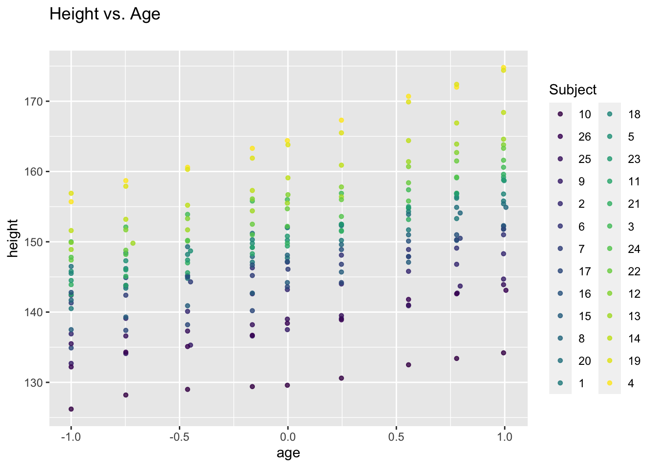

We can also have a different look at the data by drawing a line graph for each subject:

ggplot(data = Oxboys, aes(x = age, y = height, col = Subject)) +
       geom_line(linewidth = 1.2, alpha = .8) +
       labs(title = "Height vs. Age", subtitle = "by subject") +
       theme(legend.position = "none")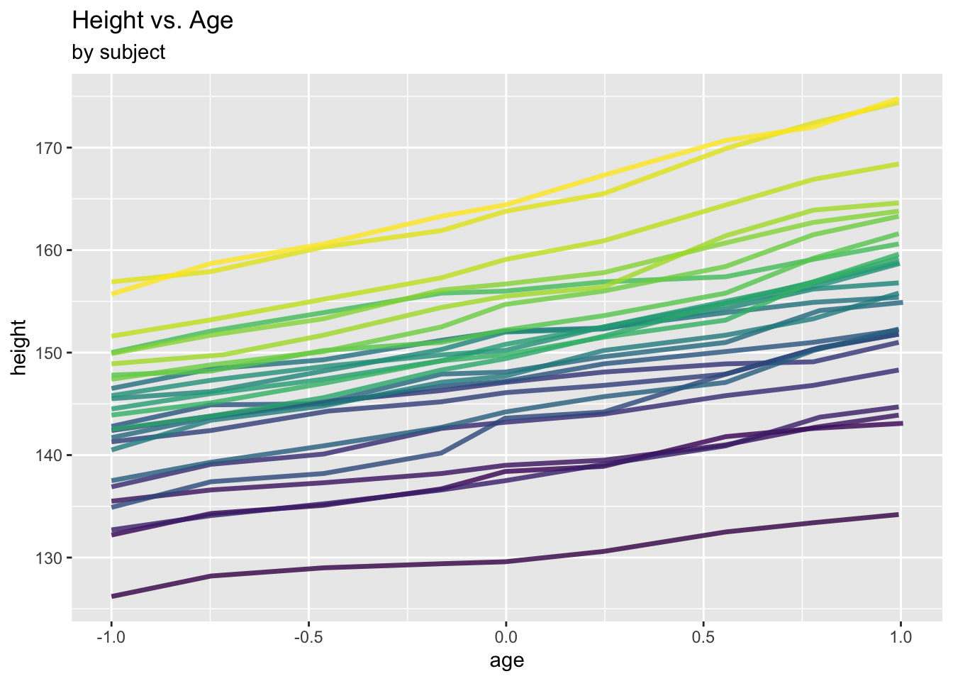

Clearly, there is within-subject correlation: measures from one subject are more similar to each other than those from different subjects.

This is a special type of repeated measures data which is commonly referred to as longitudinal data: repeated measures on certain individuals over time.

6.1.2 Example: Mathematics achievement data

The data used here represent Mathematics achievement scores of a subsample of subjects from the 1982 High School and Beyond Survey. The full dataset can be found within the package merTools.

For each of 30 schools, we have pupil-level data on Mathematics achievement and a few covariates including socioeconomic status. The data file sub_hsb.RData can be downloaded from the Ultra folder “Other Material/Term 2 Datasets”. After downloading the data, we can load and inspect it.

load("sub_hsb.RData")
head(sub_hsb)

##   schid minority female    ses mathach size schtype meanses
## 1  1224        0      1 -1.528   5.876  842       0  -0.428
## 2  1224        0      1 -0.588  19.708  842       0  -0.428
## 3  1224        0      0 -0.528  20.349  842       0  -0.428
## 4  1224        0      0 -0.668   8.781  842       0  -0.428
## 5  1224        0      0 -0.158  17.898  842       0  -0.428
## 6  1224        0      0  0.022   4.583  842       0  -0.428

dim(sub_hsb)

## [1] 1329    8

First, we plot all data points, together with a linear model fitted to the whole data set.

ggplot(data = sub_hsb, aes(x = ses, y = mathach)) +
  geom_point(size = 0.8, alpha = .8) +
  geom_smooth(method = "lm", se = FALSE, col = "Red") +
  ggtitle("Mathematics achievement vs. Socioeconomic status (SES)") +
  xlab("SES") +
  ylab("Mathematics achievement")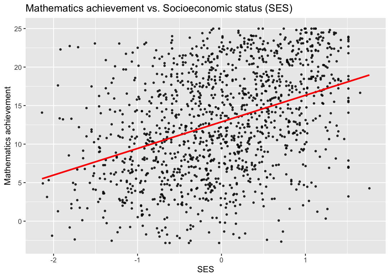

This plot shows a general trend for the whole data set, but we also would want to plot the trend for each school. To do this, we convert the school IDs into a factor with 30 levels and plot each school using a different colour.

school.id <- as.factor(sub_hsb$schid)
length(levels(school.id))

## [1] 30

ggplot(data = sub_hsb, aes(x = ses, y = mathach, colour = school.id)) +
  geom_point(size = 0.8, alpha = .8) +
  geom_smooth(method="lm", se=FALSE) +
  ggtitle("Mathematics achievement vs. Socioeconomic status (SES)",
          subtitle ="by cluster (school)") +
  xlab("SES") +
  ylab("Mathematics achievement") +
  theme(legend.position = "none")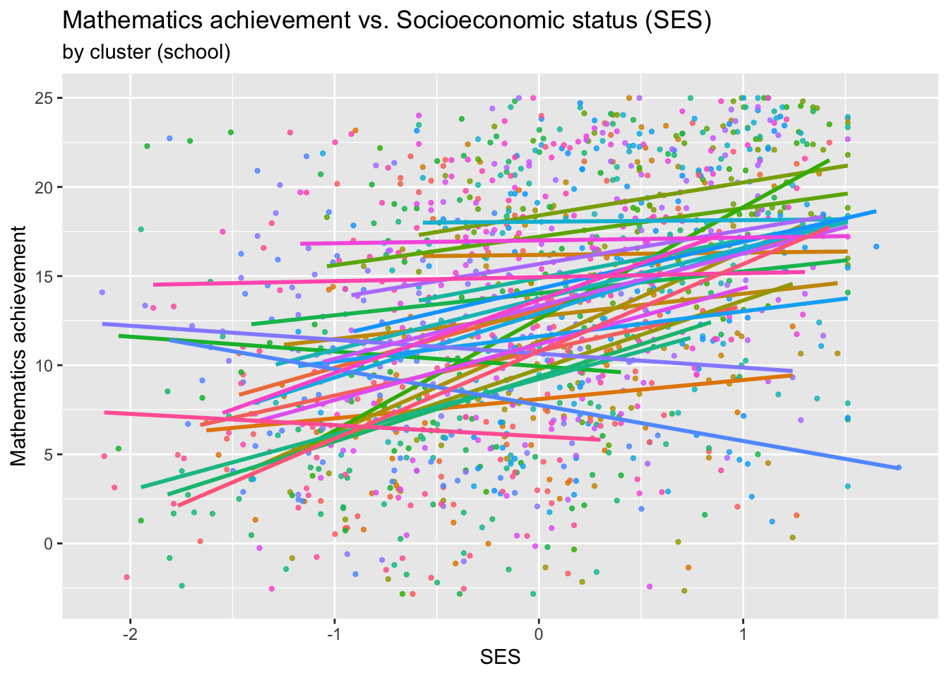

One will suspect from these plots that there is within-school correlation: pupils from one school tend to be more similar to each other than to pupils from different schools.

This type of repeated measures data is commonly referred to as “clustered” data, with clusters referring to schools. Note that the term “cluster” here should be interpreted as “items of increased similarity due to a structural reason”. It has nothing to do with “clustering”, for instance, in k-means.

Fitting naïve LMs or GLMs to repeated measures data may or may not result in correct inferences for $\boldsymbol{\beta}$ , but in any case the standard errors $SE(\hat{\beta}_j)$ will be incorrect. Fortunately, longitudinal and clustered data can be dealt with in the same framework.

6.2 Marginal model for repeated measures

Denote by $y_{ij}$ (with $i=1, \ldots, n$ and $j=1, \ldots, n_i$ ) the $j$ th repeated measurement for cluster/individual $i$ (we will just speak of “cluster” henceforth), so that the total sample size is $N=\sum_{i=1}^n n_i$ . Denote further the vector of all responses (repeated messurements) belonging to the $i$ th cluster by

$\boldsymbol{Y}_i=\left(\begin{array}{c} y_{i1}\\ \vdots \\ y_{in_i}\end{array}\right)$

with associated covariates

$\boldsymbol{X}_i= \left(\begin{array}{c} \boldsymbol{x}_{i1}^T \\ \vdots \\\boldsymbol{x}_{in_i}^T\end{array} \right) = \left(\begin{array}{ccc} x_{i11}& \ldots & x_{i1p}\\ \vdots & \ddots & \vdots \\ x_{in_i1} & \ldots & x_{in_ip} \end{array}\right).$

A marginal model for $y_{ij}$ has three components:

The mean function (assumed “correctly specified”):

$\mu_{ij}=E(y_{ij})=h(\boldsymbol{\beta}^T \boldsymbol{x}_{ij}).$

The mean-variance relationship:

$\mbox{Var}(y_{ij})=\phi \, \mathcal{V}(\mu_{ij}).$

The association between the responses:

$\begin{aligned} \mbox{corr}(y_{ij}, y_{i'k}) &= 0 \,\, \mbox{ for all } \,\, i\not=i' \\ \mbox{corr}(y_{ij}, y_{ik}) &= r_{jk} (\boldsymbol\alpha) \end{aligned}$

where $r_{jk}(\cdot)$ is a known function indexed by $j, k=1, \ldots, n_i$ and $\boldsymbol{\alpha}$ is a set of parameters of the correlation.

The specified variances and correlations of the $y_{ij}$ define uniquely the variance matrix $\boldsymbol{\Sigma}_i$ of the elements of the $i$ th cluster.

The most common settings of the function $r_{jk}(\cdot)$ are as follows:

Independence: Here $r_{jk}(\boldsymbol{\alpha}) = r_{jk}$ does not depend on parameters, where

$r_{jk} =\left\{\begin{array}{ll} 1 & j=k \\ 0 & j \not= k \end{array} \right.$

Exchangeable or equicorrelation: For $\boldsymbol{\alpha}=\alpha \in \mathbb{R}$ ,

$r_{jk}(\alpha)= \left\{ \begin{array}{ll} 1 & j=k \\ \alpha & j \not= k \end{array} \right.$

Autoregressive model (AR-1): For $\boldsymbol{\alpha}=\alpha \in \mathbb{R}$ ,

$r_{jk}(\alpha)= \alpha^{|j-k|}.$

Unstructured: Assuming $n_i = n^*$ for all $i$ , then $\boldsymbol{\alpha} \in \mathbb{R}^{n^* \times n^*}$ and

$r_{jk}(\boldsymbol{\alpha})= \boldsymbol{\alpha}_{jk}.$

Some notes:

There is no distributional assumption and there is no likelihood (Beyond the repeated measures context, this approach is also useful for complex modelling scenarios where building a likelihood may be very hard).
$\boldsymbol{\alpha}$ and $\boldsymbol{\beta}$ are overall model parameters which do not depend on the cluster, $i$ .
Marginal models provide “population-averaged” effects (unlike “conditional effects”, which provide effects conditional on each cluster $i$ , as we will see later for the mixed models).

What can we say about the variance matrices $\boldsymbol{\Sigma}_i$ ?

Firstly, element-wise, combining the specifications of variances and correlations, we have:

$\mbox{Cov}(y_{ij}, y_{ik})= \phi \, r_{jk}(\boldsymbol{\alpha}) \sqrt{\mathcal{V}(\mu_{ij})} \sqrt{\mathcal{V}(\mu_{ik})}.$

Globally, defining the working correlation matrix

$R_i(\boldsymbol{\alpha}) = (r_{jk}(\boldsymbol{\alpha}))_{1\le j \le n_i, \, 1 \le k \le n_i}$

and

$C_i(\boldsymbol{\beta}, \phi)= \mbox{diag}(\phi \, \mathcal{V}(\mu_{ij})),$

one has $\boldsymbol{\Sigma}_i=C_i^{1/2}(\boldsymbol{\beta}, \phi) \, R_i(\boldsymbol{\alpha}) \, C_i^{1/2}(\boldsymbol{\beta}, \phi),$

which clearly depends on $\boldsymbol{\alpha}$ , $\boldsymbol{\beta}$ , and $\phi$ .

6.2.1 Some examples

We exemplify the model structure through some of our recent data examples.

US Polio data (Section 5.4.1): for the model uspolio.gee3 with $\boldsymbol{x}_{ij}$ being the vector of covariates for month $j$ of year $i$ (each year is a cluster),

$\begin{aligned} \mu_{ij} &= \exp(\boldsymbol{\beta}^T \boldsymbol{x}_{ij}) \\ \mathcal{V}(\mu_{ij}) &= \mu_{ij} \\ r_{jk}(\alpha) &= \alpha^{|j-k|} \\ \mbox{Cov}(y_{ij}, y_{ik}) &= \phi \, \alpha^{|j-k|} \sqrt{\mu_{ij} \,\mu_{ik}}. \end{aligned}$

Oxford boys data (Section 6.1.1): for a model with Gaussian response, identity link, and AR-1 correlation structure,

$\begin{aligned} \mu_{ij} &= \beta_0 + \beta_1 \, \text{age}_{ij} \\ \mathcal{V}(\mu_{ij}) &= 1, \quad \mbox{where } \phi = \sigma^2 \\ r_{jk}(\alpha) &= \alpha^{|j-k|} \\ \mbox{Cov}(y_{ij}, y_{ik}) &= \sigma^2 \, \alpha^{|j-k|}. \end{aligned}$

Mathematics achievement data (Section 6.1.2): for a model with Gaussian response, identity link, and exchangeable correlation structure,

$\begin{aligned} \mu_{ij} &= \beta_0+\beta_1 \, \mbox{ses}_{ij} \\ \mathcal{V}(\mu_{ij}) &= 1, \quad \mbox{where } \phi = \sigma^2 \\ r_{jk}(\alpha) &= \left\{ \begin{array}{lc} \alpha & \mbox{if } j \not= k \\ 1 & \mbox{if } j = k \end{array} \right. \\ \mbox{Cov}(y_{ij}, y_{ik}) &= \left\{ \begin{array}{lc} \alpha \, \sigma^2 & \mbox{if } j \not= k \\ \sigma^2 & \mbox{if } j = k. \end{array} \right. \end{aligned}$

6.3 Estimation

All that is needed to estimate the model elaborated above is the (generalized version of the) quasi-score function:

$S(\boldsymbol{\beta})= \boldsymbol{X}^T\boldsymbol{D}\boldsymbol{\Sigma}^{-1}(\boldsymbol{Y}-\boldsymbol{\mu})$ where

$\boldsymbol{Y} = \left(\begin{array}{c} \boldsymbol{Y}_1 \\ \vdots \\ \boldsymbol{Y}_n \end{array}\right) \in \mathbb{R}^N, \quad \boldsymbol{X} = \left(\begin{array}{c} \boldsymbol{X}_1 \\ \vdots \\ \boldsymbol{X}_n \end{array}\right) \in \mathbb{R}^{N \times p}, \quad \boldsymbol{\mu} = \left(\begin{array}{c} \boldsymbol{\mu}_1 \\ \vdots \\ \boldsymbol{\mu}_n \end{array}\right) \in \mathbb{R}^{N},$

with $\boldsymbol{Y}_i$ and $\boldsymbol{X}_i$ defined in Section 6.2, and $\boldsymbol{\mu}_i = (\mu_{i1}, \ldots, \mu_{in_i})^T$ with $\mu_{ij}=h(\boldsymbol\beta^T \boldsymbol{x}_{ij})$ and $\boldsymbol{\beta} \in \mathbb{R}^p$ . Furthermore,

$\begin{aligned} \boldsymbol{D} &= \left(\begin{array}{cccc} h'(\boldsymbol\beta^T \boldsymbol{x}_{11}) & & & \\ & h'(\boldsymbol\beta^T \boldsymbol{x}_{12}) & & \\ & & \ddots & \\ & & & h'(\boldsymbol\beta^T \boldsymbol{x}_{nn_n}) \end{array}\right) \in \mathbb{R}^{N\times N}, \\[5pt] \boldsymbol\Sigma &= \left(\begin{array}{cccc} \boldsymbol\Sigma_1 & & & \\ & \boldsymbol\Sigma_2 & & \\ & & \ddots & \\ & & & \boldsymbol\Sigma_n \end{array}\right) \in \mathbb{R}^{N \times N}, \end{aligned}$

with $\boldsymbol\Sigma_i \in \mathbb{R}^{n_i \times n_i}$ defined in Section 6.2. Setting $S(\boldsymbol{\beta})$ to 0 yields the generalized estimating equation (GEE),

$\boldsymbol{X}^T\boldsymbol{D}\boldsymbol{\Sigma}^{-1}(\boldsymbol{Y}-\boldsymbol{\mu})=0.$

If $\boldsymbol{\Sigma}$ is known (and correctly specified) up to a multiplicative function of $\phi$ (but not depending on further parameters, $\boldsymbol{\alpha}$ ), then we can solve the GEE via Iteratively Weighted Least Squares (IWLS). That is, in complete analogy to the GLM estimation routines in Section 2.8, one has

$\hat{\boldsymbol{\beta}}_{m+1}=(\boldsymbol{X}^T\boldsymbol{D}\boldsymbol{\Sigma}^{-1}\boldsymbol{D}\boldsymbol{X})^{-1}\boldsymbol{X}^T\boldsymbol{D}\boldsymbol{\Sigma}^{-1}\boldsymbol{D}\hat{\boldsymbol{Y}}_m$

where $\hat{\boldsymbol{Y}}_m$ is a vector of working observations (which is also the same as in Section 2.8). If $\boldsymbol{Y}$ is multivariate normal and $h^{-1}(\cdot)$ is the identity link (so $\boldsymbol{D}=\boldsymbol{I}$ ), then one iteration $(\boldsymbol{X}^T\boldsymbol{\Sigma}^{-1}\boldsymbol{X})^{-1}\boldsymbol{X}^T\boldsymbol{\Sigma}^{-1}\boldsymbol{Y}$ is sufficient. In either case, estimation of $\boldsymbol{\beta}$ does not depend on $\phi$ , so $\phi$ can be estimated separately after the last iteration.

Otherwise, if $\boldsymbol{\Sigma}$ depends on unknown parameters $\boldsymbol{\alpha}$ , we cycle between:

Given current $\hat{\boldsymbol{\alpha}}$ and $\hat{\phi}$ , estimate $\hat{\boldsymbol{\beta}}$ by (one iteration of) IWLS;
Given current $\hat{\boldsymbol{\beta}}$ , estimate $\hat{\boldsymbol{\alpha}}$ and $\hat{\phi}$ [explicit formulas in Fahrmeir and Tutz (2001); page 125].

Variance estimation: Under either scenario, we can estimate the variance using one of the methods below.

“naïve”:

$\mbox{Var}(\hat{\boldsymbol{\beta}})= (\boldsymbol{X}^T\boldsymbol{D}\boldsymbol{\Sigma}^{-1}\boldsymbol{D}\boldsymbol{X})^{-1}\equiv \boldsymbol{F}^{-1}.$

“robust” (sandwich variance estimator):

$\mbox{Var}_s(\hat{\boldsymbol{\beta}})= \boldsymbol{F}^{-1}\boldsymbol{V}\boldsymbol{F}^{-1}$

where $\boldsymbol{V}=\boldsymbol{X}^T\boldsymbol{D}\boldsymbol{\Sigma}^{-1}\boldsymbol{S}\boldsymbol{\Sigma}^{-1}\boldsymbol{D}\boldsymbol{X}$ , and $\boldsymbol{S}$ is the so-called “true” variance matrix estimated as

$\boldsymbol{S}= \left(\begin{array}{ccc}\boldsymbol{S}_1 &&\\ & \ddots & \\ && \boldsymbol{S}_n \end{array}\right) \in \mathbb{R}^{N \times N},$

with $\boldsymbol{S}_i=(\boldsymbol{Y}_i-\hat{\boldsymbol{\mu}}_i)(\boldsymbol{Y}_i-\hat{\boldsymbol{\mu}}_i)^T$ .

Theoretical properties [Fahrmeir and Tutz (2001); page 126/127]: Under some regularity conditions, $\hat{\boldsymbol{\beta}}$ is consistent (i.e. $\hat{\boldsymbol{\beta}} \rightarrow \boldsymbol{\beta}^*$ for $N \rightarrow \infty$ ) and asymptotically normal,

$\hat{\boldsymbol{\beta}} \sim \mathcal{N}(\boldsymbol{\beta}^*, \boldsymbol{F}^{-1}\boldsymbol{V}\boldsymbol{F}^{-1} )$

even if the specification of $\boldsymbol{\Sigma}$ is wrong. Therefore, correct specification of $\boldsymbol{\mu}$ is more important than that of $\boldsymbol{\Sigma}$ .

6.3.1 Example

Mathematics achievement data

We fit a GEE for the Mathematics achievement data:

require(gee)
hsb.gee <- gee(mathach ~ ses, data = sub_hsb, 
               id=school.id, corstr = "exchangeable")

## Beginning Cgee S-function, @(#) geeformula.q 4.13 98/01/27

## running glm to get initial regression estimate

## (Intercept)         ses 
##   12.886358    3.453019

hsb.gee

## 
##  GEE:  GENERALIZED LINEAR MODELS FOR DEPENDENT DATA
##  gee S-function, version 4.13 modified 98/01/27 (1998) 
## 
## Model:
##  Link:                      Identity 
##  Variance to Mean Relation: Gaussian 
##  Correlation Structure:     Exchangeable 
## 
## Call:
## gee(formula = mathach ~ ses, id = school.id, data = sub_hsb, 
##     corstr = "exchangeable")
## 
## Number of observations :  1329 
## 
## Maximum cluster size   :  67 
## 
## 
## Coefficients:
## (Intercept)         ses 
##   12.884541    2.170503 
## 
## Estimated Scale Parameter:  41.85127
## Number of Iterations:  4
## 
## Working Correlation[1:4,1:4]
##           [,1]      [,2]      [,3]      [,4]
## [1,] 1.0000000 0.1253383 0.1253383 0.1253383
## [2,] 0.1253383 1.0000000 0.1253383 0.1253383
## [3,] 0.1253383 0.1253383 1.0000000 0.1253383
## [4,] 0.1253383 0.1253383 0.1253383 1.0000000
## 
## 
## Returned Error Value:
## [1] 0

We plot the fitted responses (blue line) and compare them with the linear model fits (red line).

sub_hsb$pred1 <- predict(hsb.gee)

ggplot(data = sub_hsb, aes(x = ses, y = mathach)) +
  geom_point(size = 0.8, alpha = .8) +
  geom_smooth(method = "lm", se = FALSE, col = "Red") +
  geom_line(aes(x = ses, y = pred1), col = "Blue") +
  ggtitle("Mathematics achievement vs. Socioeconomic status (SES)",
          subtitle = "Blue line is GEE solution") +
  xlab("SES") +
  ylab("Mathematics achievement")

## `geom_smooth()` using formula = 'y ~ x'

What about standard errors?

summary(hsb.gee)$coef

##              Estimate Naive S.E.   Naive z Robust S.E. Robust z
## (Intercept) 12.884541  0.4524909 28.474697   0.4784090 26.93206
## ses          2.170503  0.2538904  8.548976   0.3576248  6.06922

We compare to standard errors of the linear model:

hsb.lm <- lm(mathach ~ ses, data = sub_hsb)
summary(hsb.lm)$coef

##              Estimate Std. Error  t value     Pr(>|t|)
## (Intercept) 12.886358  0.1752970 73.51156 0.000000e+00
## ses          3.453019  0.2222153 15.53907 3.738528e-50

Observations:

Both the actual estimates, and their standard errors, are quite different for the GEE and the LM.
The robust standard errors are still a bit larger than the naive ones.

Oxford boys data

We fit GEE for Oxford boys data:

data(Oxboys, package="nlme")
oxboys.gee <- gee(height~age, data=Oxboys, id=Subject, corstr="AR-M", Mv=1)

## Beginning Cgee S-function, @(#) geeformula.q 4.13 98/01/27

## running glm to get initial regression estimate

## (Intercept)         age 
##  149.371801    6.521022

oxboys.gee

## 
##  GEE:  GENERALIZED LINEAR MODELS FOR DEPENDENT DATA
##  gee S-function, version 4.13 modified 98/01/27 (1998) 
## 
## Model:
##  Link:                      Identity 
##  Variance to Mean Relation: Gaussian 
##  Correlation Structure:     AR-M , M = 1 
## 
## Call:
## gee(formula = height ~ age, id = Subject, data = Oxboys, corstr = "AR-M", 
##     Mv = 1)
## 
## Number of observations :  234 
## 
## Maximum cluster size   :  9 
## 
## 
## Coefficients:
## (Intercept)         age 
##  149.719096    6.547328 
## 
## Estimated Scale Parameter:  65.41743
## Number of Iterations:  2
## 
## Working Correlation[1:4,1:4]
##           [,1]      [,2]      [,3]      [,4]
## [1,] 1.0000000 0.9892949 0.9787045 0.9682274
## [2,] 0.9892949 1.0000000 0.9892949 0.9787045
## [3,] 0.9787045 0.9892949 1.0000000 0.9892949
## [4,] 0.9682274 0.9787045 0.9892949 1.0000000
## 
## 
## Returned Error Value:
## [1] 0

We plot and compare to linear model:

Oxboys$pred1 <- predict(oxboys.gee)

ggplot(data = Oxboys, aes(x = age, y = height, col = Subject)) +
  geom_point(size = 1.2, alpha = .8) +
  geom_smooth(method="lm", se=FALSE, col="Red") +
  geom_line(aes(x = age, y = pred1), col="Blue") +
  labs(title = "Height vs. Age", subtitle="Blue line is GEE solution") +
  theme(legend.position = "none")

## `geom_smooth()` using formula = 'y ~ x'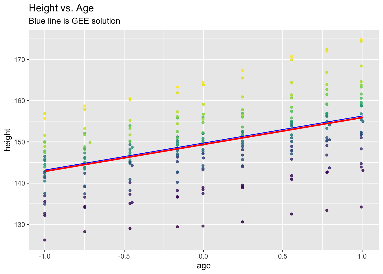

We also compare standard errors:

summary(oxboys.gee)$coef

##               Estimate Naive S.E.  Naive z Robust S.E. Robust z
## (Intercept) 149.719096  1.5531285 96.39840   1.5847569 94.47449
## age           6.547328  0.3177873 20.60286   0.3042478 21.51972

oxboys.lm <- lm(height~age, data=Oxboys)
summary(oxboys.lm)$coef

##               Estimate Std. Error    t value      Pr(>|t|)
## (Intercept) 149.371801  0.5285648 282.598864 1.987406e-296
## age           6.521022  0.8169867   7.981797  6.635134e-14

Standard errors under the GEE can also decrease!

In general, standard errors under GEEs with non-independent data assumption (e.g., with exchangeable or AR(1) correlation structure) can be larger or smaller than those with independent data assumption (e.g., in linear models or standard GLMs). See exercise 4 of this chapter for an example.

6.4 Exercises

Question 1

Explain why the quasi-likelihood method in Section 5.3 is a special case of marginal models.
Consider the R code below for the US Polio data. Explain why the estimated coefficients and (naive) standard errors are the same for these models.
Explain why the robust standard errors are different in the polio.m2 and polio.m3 models.

polio.m1 <- glm(cases~time, family=quasipoisson, data=uspolio)
polio.m2 <- gee(cases~time, family=poisson, id=rep(1,168),
                corstr = "independence", data=uspolio)
polio.m3 <- gee(cases~time, family=poisson, id=1:168,
                corstr = "exchangeable", data=uspolio)

summary(polio.m1)$coef
summary(polio.m2)$coef
summary(polio.m3)$coef

Question 2

Let $y_t$ follow an $AR(1)$ process such that:

$y_t = \alpha \, y_{t-1} + \epsilon_t \,\, \mbox{ with } \,\, \epsilon_t \sim \mathcal{N}(0, \sigma^2).$

Show that $\mbox{Corr}(y_t, y_{t+1}) = \alpha$ .

Note: You can restrict to the case $|\alpha|<1$ and use without proof the fact that in this case the AR(1) process is stationary; particularly, the $y_t$ ’s possess constant variance.

For a certain longitudinal dataset, we assume AR(1) correlation structure within subjects, and independence between subjects. The execution of a GEE with the corresponding variance structure yields an estimate of the working correlation matrix below. What is the estimate of $\alpha$ ?

Working Correlation[1:4,1:4]
           [,1]       [,2]       [,3]       [,4]
[1,] 1.00000000 0.30346880 0.09209331 0.02794745
[2,] 0.30346880 1.00000000 0.30346880 0.09209331
[3,] 0.09209331 0.30346880 1.00000000 0.30346880
[4,] 0.02794745 0.09209331 0.30346880 1.00000000

Question 3

Consider a model $\boldsymbol{Y} \sim \mathcal{N}(\boldsymbol\mu, \boldsymbol\Sigma)$ , where $\boldsymbol{Y} \in \mathbb{R}^N$ , $\boldsymbol\mu = \boldsymbol{X} \boldsymbol\beta$ with $\boldsymbol{X} \in \mathbb{R}^{N \times p}$ and $\boldsymbol\beta \in \mathbb{R}^p$ , and a positive definite matrix $\boldsymbol{\Sigma} \in \mathbb{R}^{N \times N}$ .

Show that

$\hat{\boldsymbol\beta} = (\boldsymbol{X}^T \boldsymbol\Sigma^{-1} \boldsymbol{X})^{-1} \boldsymbol{X}^T \boldsymbol\Sigma^{-1} \boldsymbol{Y}$ solves the estimating equation

$\boldsymbol{X}^T \boldsymbol\Sigma^{-1} (\boldsymbol{Y} - \boldsymbol{\mu}) = 0.$

Find an expression for $\mbox{Var}(\hat{\boldsymbol\beta})$ , simplifying as far as possible.
Assume the matrix $\boldsymbol\Sigma$ is fully known up to a dispersion parameter. Explain why the estimator $\hat{\boldsymbol\beta}$ from part (a) can be used without estimating that dispersion.
Consider a situation with $N=6$ , where three repeated measures have been taken from each of two individuals. Sketch an appropriately parameterized matrix $\boldsymbol\Sigma$ for this scenario, assuming we do not want to account for temporal autocorrelations.

Question 4

Consider repeated measures data of $n$ individuals where there are two observations $y_{i1}$ and $y_{i2}$ for each individual $i$ . Let there be a single covariate $x_{ij} \in \mathbb{R}$ for $i \in \{ 1, \ldots, n \}$ and $j \in \{ 1, 2 \}$ . Consider fitting a marginal model with Gaussian response, exchangeable (or equivalently, AR-1) correlation structure, and linear predictor $\eta_{ij} = \beta \, x_{ij}$ without an intercept.

Specify the matrices $\boldsymbol{X}$ , $\boldsymbol{Y}$ , $\boldsymbol{D}$ , $\boldsymbol\Sigma$ , and their dimensions.
Derive an explicit expression for the naive $\text{Var}(\hat\beta)$ in terms of $\hat\beta$ , $h$ , $\hat\alpha$ , $\hat\sigma$ , and $x_{ij}$ ’s.
Consider the case where $x_{i1} = x_{i2}$ for all $i$ (e.g., $x_{ij}$ could be an indicator of whether the individual is native-born). Show that if $\hat\alpha > 0$ , then $\text{Var}(\hat\beta)$ is larger compared to when $\hat\alpha = 0$ , assuming $\hat\beta$ and $\hat\sigma$ are the same in both cases.
Consider the case where $x_{i1} = 0$ and $x_{i2} \neq 0$ for all $i$ (e.g., when we collected data before and after an event and $x_{ij}$ is the indicator of whether the event had occurred). Show that if $0 < \hat\alpha < 1$ , then $\text{Var}(\hat\beta)$ is smaller compared to when $\hat\alpha = 0$ , assuming $\hat\beta$ and $\hat\sigma$ are the same in both cases.

Question 5

(Adapted from Dobson & Barnett, 2018)

Suppose that $(Y_{ij}, x_{ij})$ are observations on the $j$ th subject in cluster $i$ (with $i= 1, \ldots, n$ and $j = 1, \ldots, m$ ) and the goal is to fit a “regression through the origin” model:

$E(Y_{ij}) = \beta x_{ij},$

where the variance-covariance matrix for $Y$ ’s in the same cluster is

$\boldsymbol{\Sigma}_i = \sigma^2 \left(\begin{array}{cccc} 1 & \rho & \dots & \rho \\ \rho & 1 & \dots & \rho \\ \vdots & \vdots & \ddots & \vdots \\ \rho & \rho & \dots & 1 \end{array}\right)$

and $Y$ ’s in different clusters are independent.

From Section 6.3, we know that if the $Y$ ’s are normally distributed, then $\hat{\boldsymbol\beta} = (\boldsymbol{X}^T\boldsymbol{\Sigma}^{-1}\boldsymbol{X})^{-1}\boldsymbol{X}^T\boldsymbol{\Sigma}^{-1}\boldsymbol{Y}$ . Show that

$\hat{\boldsymbol\beta} = \big( \sum_{i=1}^n \boldsymbol{x}^T_i \boldsymbol{\Sigma}_i^{-1} \boldsymbol{x}_i \big)^{-1} \big( \sum_{i=1}^n \boldsymbol{x}^T_i \boldsymbol{\Sigma}_i^{-1} \boldsymbol{y}_i \big) \;\; \text{ with } \;\; \text{Var}(\hat{\boldsymbol\beta}) = \big( \sum_{i=1}^n \boldsymbol{x}^T_i \boldsymbol{\Sigma}_i^{-1} \boldsymbol{x}_i \big)^{-1},$

where $\boldsymbol{x}_i = (x_{i1}, \ldots, x_{im})^T$ and $\boldsymbol{y}_i = (y_{i1}, \ldots, y_{im})^T$ . Also deduce that the estimate $\hat{\beta}$ of $\beta$ is unbiased.

$\boldsymbol{\Sigma}_i^{-1} = c \left(\begin{array}{cccc} 1 & \phi & \dots & \phi \\ \phi & 1 & \dots & \phi \\ \vdots & \vdots & \ddots & \vdots \\ \phi & \phi & \dots & 1 \end{array}\right)$

where

$c = \frac{1}{\sigma^2(1 + (m-1)\phi\rho)} \;\; \text{ and } \;\; \phi = \frac{-\rho}{1 + (m-2)\rho},$

show that

$\text{Var}(\hat{\beta}) = \frac{\sigma^2(1 + (m-1)\phi\rho)}{\sum_i \left\{ \sum_j x_{ij}^2 + \phi \left[ (\sum_j x_{ij})^2 - \sum_j x_{ij}^2 \right] \right\} }.$

If the clustering is ignored, show that the estimate $b$ of $\beta$ has $\text{Var}(b) = \sigma^2/\sum_i \sum_j x_{ij}^2$ .
If $\rho = 0$ , show that $\text{Var}(\hat\beta) = \text{Var}(b)$ as expected if there is no correlation within clusters.
If $\rho = 1$ , $\boldsymbol{\Sigma}_i/\sigma^2$ is a matrix of ones, so the inverse does not exist. But the case of maximum correlation is equivalent to having just one element per cluster. If $m=1$ , show that $\text{Var}(\hat\beta) = \text{Var}(b)$ in this situation.
If the study is designed so that $\sum_j x_{ij} = 0$ and $\sum_j x_{ij}^2$ is the same for all clusters, let $W = \sum_i \sum_j x_{ij}^2$ and show that

$\text{Var}(\hat{\beta}) = \frac{\sigma^2(1 + (m-1)\phi\rho)}{W(1-\phi)}.$

With this notation, $\text{Var}(b) = \sigma^2/W$ ; hence, show that

$\frac{\text{Var}(\hat\beta)}{\text{Var}(b)} = \frac{1 + (m-1)\phi\rho}{1-\phi} = 1 - \rho.$

Deduce the effect on the estimated standard error of the slope estimate for this model if the clustering is ignored.

References

Fahrmeir, Ludwig, and Gerhard Tutz. 2001. Multivariate Statistical Modelling Based on Generalized Linear Models (2nd Edition). Springer.