Vignette 5 Evaluation by simulation

Gates Dupont & Chris Sutherland

5.1 Simulating SCR data

We can evaluate a design by simulating data and recovering parameter estimates.

We illustrate this using simulator(), which executes the following:

1. Randomly assigns N activity centers to the state-space
2. Calculates \(p\) for each \((x, s_i)\) pair based on distance
3. Creates a 3D encounter history array, \([i,j,k]\), using a binomial model
4. Fits a basic SCR model using oSCR.fit()
5. Returns parameter estimates and summary statistics

Here’s the simulation function that we use. It’s fairly straightforward, but has a few extra elements to help with troubleshooting.

require(oSCR)
require(dplyr)

simulator<- function(traps, ss, N, p0, sigma, K, nsim, plot = TRUE) {
  
  # Initialize data-collection matrix
  simout1 <- matrix(NA, nrow=0, ncol=9)                   # Create empty matrix for output
  colnames(simout1)<- c("p0","sig","d0",                  # Estimates
                        "nind",                           # Number of individuals (length of first dimmension of y)
                        "avg.caps","avg.spatial","mmdm",  # Summary stats from oSCR (possibly different definitions)
                        "failures","EN")                  # Other components
  
  # Initialize while loop starting values
  sim = 1         # Starting value for nsim
  sim_try = 0     # Feature to aid in tracking failures
  total_its = 0   # Feature to insure different random seeds
  
  # Get nsim "good" simulations (no failures)
  while(sim < (nsim + 1)){
    
    # Update loop for seed
    total_its = total_its + 1
    
    # Update status
    print(paste("Simulation Number", sim, sep = " ")) # keep track
    cat("size of state-space: ", nrow(ss), " pixels", fill=TRUE)
    cat(paste0("\n Try ", sim_try + 1, "\n"))
    
    # Re-assign name
    statespace = ss
    
    # Set seed for simulation
    seed = total_its
    set.seed(seed)
    
    # Sampling activity centers
    s <- statespace[base::sample(x = nrow(statespace), size = N),]
    
    # Make the state space data frame (oSCR object)
    myss <- as.data.frame(statespace)
    myss$Tr <- 1
    myss <- list(myss)
    class(myss) <- "ssDF"
    
    # Individual-trap distance matrix
    D <- e2dist(s,traps)
    
    # Compute detection probabilities:
    pmat <- p0*exp(-D*D/(2*sigma*sigma)) # p for all inds-traps p_ij
    ntraps <- nrow(traps)
    
    # Setup encounter histories data frames
    y <- array(0, dim=c(N, ntraps, K)) # empty 3D array (individuals by traps by sampling occasion)
    
    # Simulate encounter histories
    for(i in 1:N){                            # loop through each individual/activity center
      for(j in 1:ntraps){                     # loop through each trap
        y[i,j,1:K]<- rbinom(K, 1, pmat[i,j])  # y ~ binomial(p_ijk)
      }
    }
    
    # Reduce encounter histories to only captured individuals
    ncap <- apply(y,c(1), sum)       # sum of captures for each individual
    y.all = y                        # for summary stats
    y <- y[ncap>0,,]                 # reduce the y array to include only captured individuals
    
    # Some summary information, which is actually printed for you later with "print(scrFrame)"
    caps.per.ind.trap <- apply(y,c(1,2),sum) # shows # capts for each indvidual across all traps
    
    # Check for captures
    check.y = length(dim(y)) %>%
      if(. > 2){return(TRUE)} else {return(FALSE)}
    
    # Check for spatial recaps
    check.sp_recaps = as.matrix((caps.per.ind.trap > 0) + 0) %>%
      rowSums() %>%
      c(.,-1) %>%    # This is just to avoid warning messages due to empty lists
      max %>%
      if(. > 1){return(TRUE)} else {return(FALSE)}
    
    # Check should be 2 if the design obtained at least a capture AND a spatial recapture
    check = 0 # Clear this value from previous iteration
    check = check.y + check.sp_recaps
    
    # Note: Checking for sp.recaps implies getting caps, 
    # but for troubleshooting good to keep both checks
    
    if(check == 2){
      
      # Make the SCRframe object
      colnames(traps) <- c("X","Y")
      sf <- make.scrFrame(caphist=list(y), traps=list(traps))
      
      # Plotting
      if(plot == TRUE){
        
        # Make plot
        plot(statespace, asp = 1, pch = 15, col = "gray85", cex = 0.9)
        points(s, pch = 20, col = "blue", cex = 0.5)
        spiderplot(sf, add=TRUE) # This plots captures and spatial recaptures between traps
        
      }
      
      # Fit a basic model SCR0 (null model, ~1 ~1 ~1)
      out1 <- oSCR.fit(model=list(D~1,p0~1,sig~1), scrFrame = sf, ssDF=myss, trimS = 4*sigma)
      
      # Obtain estimates from the model
      stats <- print(sf)[[1]]   # pulls avg caps, avg spatial caps, and mmdm
      est <- out1$outStats$mle  # pulls p0, sigma, and d0 estimates from the model
      en = get.real(out1, type="dens", newdata=data.frame(session=factor(1)),
                    d.factor=nrow(out1$ssDF[[1]]))[1,1] # Total abundance
      
      # Append to data-collection matrix
      sim_vals = c(plogis(est[1]), exp(est[2]), exp(est[3]), dim(y)[1], stats, sim_try, en)
      simout1 = rbind(simout1, sim_vals)
      
      # Just add two blank lines to live status updates
      cat("\n\n")
      
    }
    
    # Updating while() loop
    if(check != 2){
      sim_try <- sim_try + 1
    } else {
      sim <- sim + 1
      sim_try = 0
    }
    
    
  }
  
  # Return the resultis from the simulation
  result = data.frame(simout1)
  return(result)
  
}

5.2 Run simulations

Running the simulations is straightforward with simulator().

# Assign study are ojbects
ss <- statespace
traps <- testdesign$optimaltraps # "traps" refers to the design in simulator()

# Assign simulation values
beta0      <- 0.025
K          <- 5
p0_sim     <- exp(beta0)/K
sigma_sim  <- 3.250
N_sim      <- 300

# Simulate using same parameter values as design
simout <- simulator(
  traps = traps, ss = ss, K = K, 
  p0 = p0_sim, sigma = sigma_sim, N = N_sim, 
  nsim = 50, # We recommend using at least `nsim=50`, or preferably more.
  plot = TRUE
)

5.3 Evaluate the results

One of the most immediately interpretable evaluation metrics is percent relative bias (“%RB”), shown below, calculated for each parameter.

\[ \%RB = 100 \sum{\frac{\hat{y} - y}{y}} \]

Other useful metrics include (though not limited to):

• coefficient of variation (precision)
• scaled root mean squared error (accuracy)
• coverage

library(tidyr)

# Evaluate
df <- data.frame(
  p0 =  100*((simout$p0-p0_sim)/p0_sim),
  sigma =  100*((simout$sig-sigma_sim)/sigma_sim),
  N =  100*((simout$EN-N_sim)/N_sim)) %>%
  gather(key = "parameter") %>%
  mutate(parameter = factor(parameter, levels = c("p0", "sigma", "N")))

5.4 Plot the evaluations

This design performs well on average for bias. Precision would improve with more traps.

ggplot(data = df, aes(x = parameter, y = value)) +
  geom_boxplot(fill = "lightblue1", color = "skyblue4", width = 0.1) + 
  geom_hline(yintercept = c(-5, 5), linetype = "dashed", color = "gray70") +
  geom_hline(yintercept = 0, lwd = 1, color = "gray70") +
  xlab(NULL) + ylab("%RB") + ylim(-100, 100) +
  theme_pubr() + theme(legend.position = "none")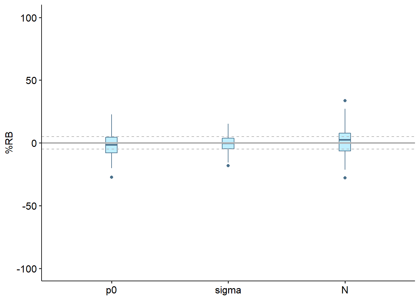

5.5 Take-home points

The oSCR framework:

• Conceptual and analytical framework for generating optimized designs.
• Three intuitive and statistically-grounded design criteria.
• Produce a greater amount of expected information, leading to more accurate estimates.
• Flexible for application to any species in any study area using SCR.

Johnson, Devin S, Dana L Thomas, Jay M Ver Hoef, and Aaron Christ. 2008. “A General Framework for the Analysis of Animal Resource Selection from Telemetry Data.” Biometrics 64 (3): 968–76.

Linden, Daniel W, Alexej PK Sirén, and Peter J Pekins. 2018. “Integrating Telemetry Data into Spatial Capture–Recapture Modifies Inferences on Multi-Scale Resource Selection.” Ecosphere 9 (4): e02203.

Royle, J Andrew, Richard B Chandler, Catherine C Sun, and Angela K Fuller. 2013. “Integrating Resource Selection Information with Spatial Capture–Recapture.” Methods in Ecology and Evolution 4 (6): 520–30.

Sun, Catherine. 2014. “Estimating Black Bear Population Density in the Southern Black Bear Range of New York with a Non-Invasive, Genetic, Spatial Capture-Recapture Study.” Master’s Thesis. Ithaca, New York, USA: Cornell University.