Vignette 4 Generating designs
Gates Dupont & Chris Sutherland
Now with data, we can demonstrate the design-generation process using our novel framework. This framework employs a genetic algorithm to solve the k-of-n problem of trap selection according to one of the previously described design criteria, which are considered to be possible study objectives for selection by the user. For more detail on the genetic algorithim, we refer the reader to Wolters et al. (2015), as well as Appendix S1 in Dupont et al. (2020), which describes the algorithm in this context. The most important details, however, will be described below.
4.1 Initial setup and parameterization
Before getting started, a few packages should be loaded:
library(oSCR)      # Design-generating function
library(kofnGA)    # Genetic algorithm backend
library(sf)        # Spatial data manipulation
library(raster)    # Raster data manipulation
library(ggplot2)   # Improved plotting
library(viridis)   # Color palette
Again, we can inspect the state-space and all possible trap locations to make sure they line up:
plot(statespace, asp=1, pch=20, cex = 0.5, col="gray65")
points(alltraps, pch=20, cex = 0.5, col = "blue")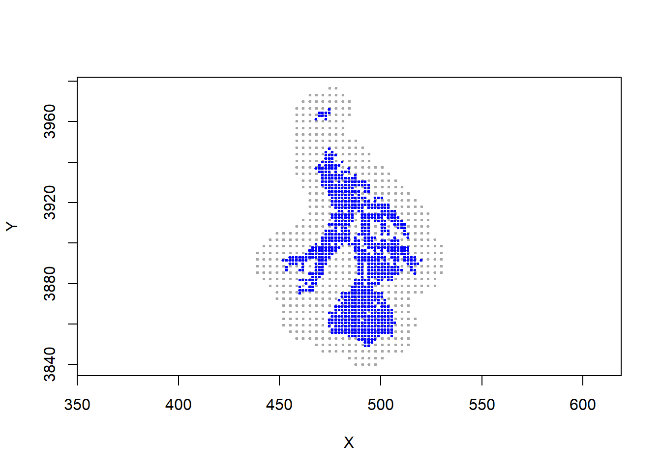
We also need values for the SCR paramters for the species of interest. These values could be optained form the literature or from a pilot study. We’ll use the same paramters as those used in the previous section.
For refernce, you can derive beta0 from the baseline encounter probability, \(p_0\), and the number of sampling occassions, \(K\).
# For reference, beta0 is log(p0 * K)
# So, we can solve for p0
tmp <- exp(beta0)   # tmp is p0 * K
K <- 5              # So, for example, assume 5 sampling occasions
p0 <- tmp/K         # Baseline encounter probability
print(p0)
## [1] 0.205063Finally, we need to determine the number of traps available for inclusion in the design.
4.2 Design-finding algorithm
Now that we have everything in place, we can run the design-finding algorithm. This is a toy exammple of what the paramterization should look like, followed by a more robust specification below. Here we use popsize = 50, keepbest = 5, and ngen = 50. In brief, the genetic algorithm is in the broader class of evolutionary algorithms, and borrows from evolutionary biology: popsize is the number of randonly-generated designs per generation, keepbest determines how many of those to keep for each generation (0.1 survival probability here), abd ngen is the number of generations to run, during which the design will “evolve.”
testdesign <- scrdesignGA(
    statespace = statespace, alltraps = alltraps, # Study area components
    ntraps = ntraps,                              # Number of available traps
    beta0 = beta0,                                # Expected data (where beta0 = log(p0 * k)
    sigma = sigma,                                # Expected data
    crit = 2,                                     # Design criterion   1) Qp    2) Qpm    3) Qpb
    popsize = 50, keepbest = 5, ngen = 50,        # Genetic algorithm settings
    verbose = F                                   # Set verbose = T to track iterations
)
Now with the design complete, we can display 3 diagnostic plots:
par(mfrow=c(1,3))             # Prep to plot 3 things
plot(testdesign, which = 4)   # Display all 3 diagnostic plots (which = 4)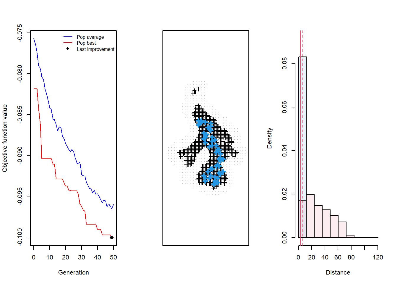
The critical thing to notice here is that the algorithm did not converge on a an “optimal” design, which we know given that the red line, labelled “Pop best”, has yet to reach a clear minimum value maintained across many generations. Further, the middle plot showing the design output seems to lack any apparent pattern in it’s structure, suggesting the process hasn’t reached completion. This might not be obvious at first, but wil become more noticeable and intuitive after spending more time using the function.
4.3 Supply a cluster to the algorithm
The lack of convergance means that we have to allow the algorithm to run for many more generations in order to find an “optimal” solution. According to Wolters et al. (2015), it’s best to set ngen to 1500+ generations, which we have also confirmed with our own testing. Running the algorithm for so many generations certainly takes a bit longer, but to speed it up we can supply a cluster to the function and parallelize the process. Depending on your machine, this can greatly reduce the amount of time it takes to generate a design. We suggest using 1500 generations for generating the final design, along with bumping up popsize to 200 and keepbest to 10% of that, or here, 20. However, if you find that the algorithm will take far too long to finish on your machine, you can bump popsize back down to 50, and likewise, keepbest down to 5. Although this isn’t considered best practice, we have yet to come across substaintially different results using those settings.
library(doParallel) # For parallelization

# Cluster setup
ncores = detectCores() - 2 # Number of available cores -1 to leave for computer
cl = makeCluster(ncores) # Make the cluster with that many cores
clusterExport(cl, varlist = c("e2dist"), envir = environment()) # Export required function to the cores

# Generate design leveraging cluster
testdesign <- scrdesignGA(
    statespace = statespace, alltraps = alltraps, # Study area components
    ntraps = ntraps,                              # Number of available traps
    beta0 = beta0,                                # Expected data (where beta0 = log(p0 * k)
    sigma = sigma,                                # Expected data
    crit = 2,                                     # Design criterion   1) Qp    2) Qpm    3) Qpb
    popsize = 50, keepbest = 5, ngen = 1500,      # Genetic algorithm settings
    cluster = cl,                                 # Use the cluster
    verbose = T                                   # Set verbose = T to track iterations
)

# Important! Remember to stop the cluster.
stopCluster(cl)
# Diagnostics plot
par(mfrow=c(1,3)) # Prep to plot 3 things
plot(testdesign, which = 4) # Display all 3 diagnostic plots (which = 4)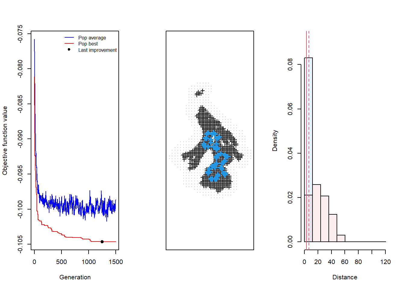
Here we see that the design has converged after around 1100 generations, with the red line bottoming-out over the course of those last 400 generations, and the resulting design appears to exhibit the structural chracteristics that we expect from the Qpm criteria. It’s worth taking a minute to compare the last two sets of plots to get a better understanding of how to know when your design has converged.
We describe the strcutral characteristics of designs from each criteria as follows: for Qp, that would be space-filling, space-constraining for Qpm (explored in this example), and clustered space-filling for Qpb. The third plot shows a histogram of trap spacing relative to sigma, which is informative about the possible resolution of the design in capturing the value of sigma. In the case of the design we generated, resolution for capturing sigma should be comprehensive, given the variation in trap spacing.
Once we have a final design, we recommend evaluating its performance using simulation, as done in Dupont et al. (2020).