Vignette 2 Design criteria
The process of optimal design for SCR is comprised of two components: a set of possible sampling locations, and an optimization criteria for selecting among those locations. In this way, the selection of an optimization criteria is critical to the end result of the study design.
2.1 Explanation of criteria
Here we describe two fundamental criteria, \(Q_{\bar{p}}\) and \(Q_{\bar{p}_{m}}\), as well as a third, \(Q_{\bar{p}_{b}}\), which is simply the sum of the two prior. At their foundation, \(Q_{\bar{p}}\) and \(Q_{\bar{p}_{m}}\) are entirely model-based, meaning that they are derived directly from the null SCR model, making for an explicit and logical relationship between design and estimation. More specifically, the criteria we propose are derived from the standard encounter process model in SCR. For a full and detailed explanation of the math behind these criteria, see Dupont et al. (2020). In summary:
2.2 Mathematical basis of criteria
To calculate these criteria, we start by calculating the probability that an individual at an activity center is detected in any trap (i.e., marginalized over all traps), \(\bar{p}(s_i,{\cal{X}})\). We then average this over all possible activity center locations (i.e., pixels in the state-space) to calculate \(\bar{p}({\cal{X}})\), which we denote simply as \(\bar{p}\).
Now that we have \(\bar{p}\), we calculate \(\bar{p}_{m}\) by subtracting from 1 two values: the probability of an individual not being captured, \(\bar{p}_0(s_i,{\cal{X}})\), and the probability of an individual being captured in just one trap, \(\bar{p}_1(s_i,{\cal{X}})\). To do this, the probability of an individual not being captured is 1 minus the probability of an individual being captured at any trap: \(1 - \bar{p}(s_i,{\cal{X}})\) (see above). Next, the probability of an individual being captured in exactly one trap is the ratio of an individual being captured to 1 minus that value, summed across all traps, and multiplied by the probability of not being captured (as previously described).
Computationally, the genetic algorithm optimizes by finding the minimum value of a given criteria, so to create \(Q_{\bar{p}}\) and \(Q_{\bar{p}_{m}}\) we assign the negative of \(\bar{p}\) and \(\bar{p}_{m}\) to their respective criterion:
\(Q_{\bar{p}} = -\bar{p}({\cal{X}})\)
\(Q_{\bar{p}_{m}} = -\bar{p}_{m}({\cal{X}})\)
Following this, \(Q_{\bar{p}_{b}}\) is the result of summing those two criteria:
- \(Q_{\bar{p}_{b}} = Q_{\bar{p}} + Q_{\bar{p}_{m}}\).
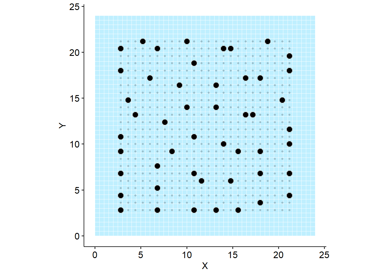
2.3 Criteria 1: space-filling
Selects for “space-filling” by optimizing for the probability of a capture.
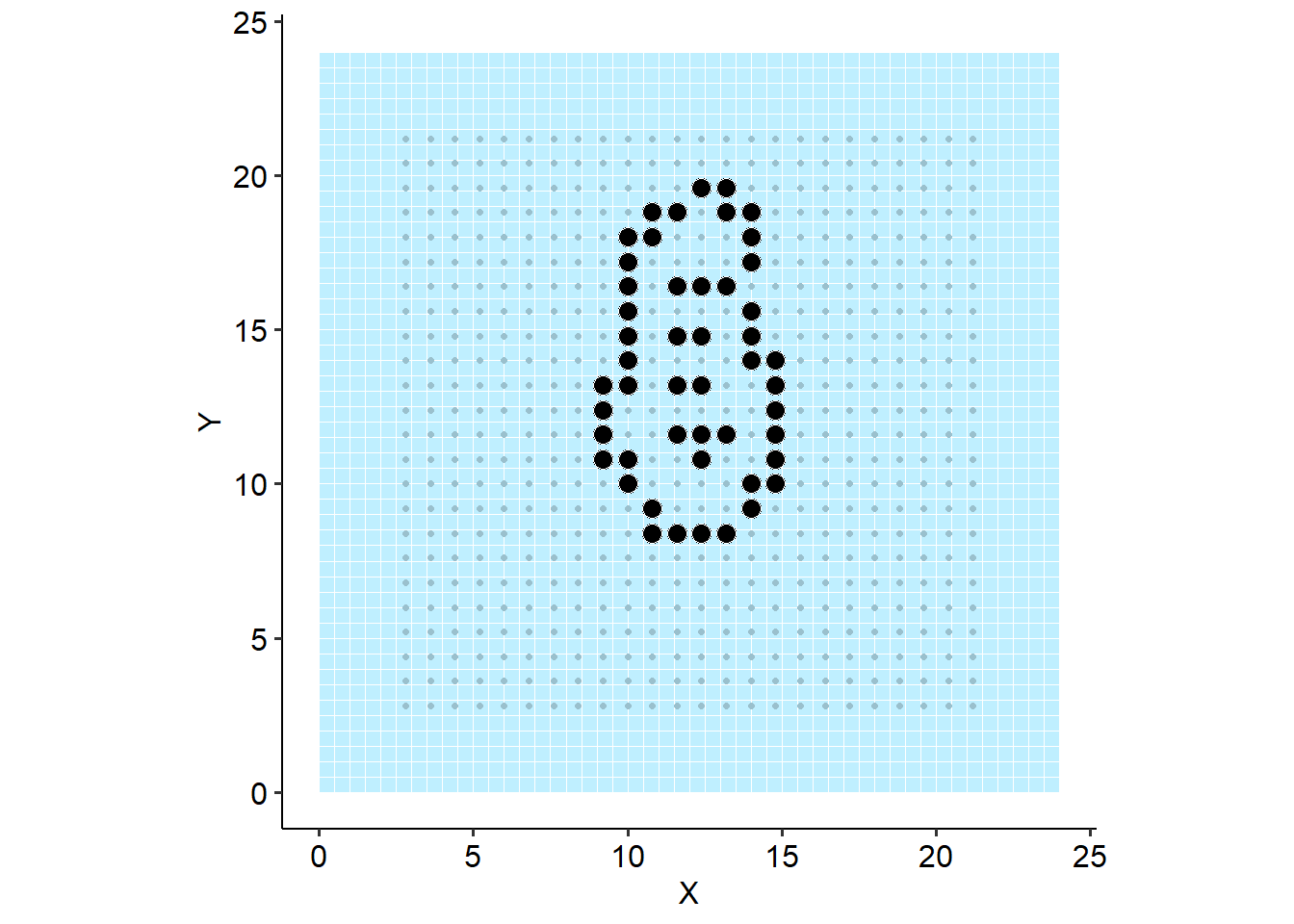
2.4 Criteria 2: space-constraining
Selects for “space-restricting” (tight clustering) by optimizing for the probability of capture at more than one trap (a.k.a., a movement recapture).
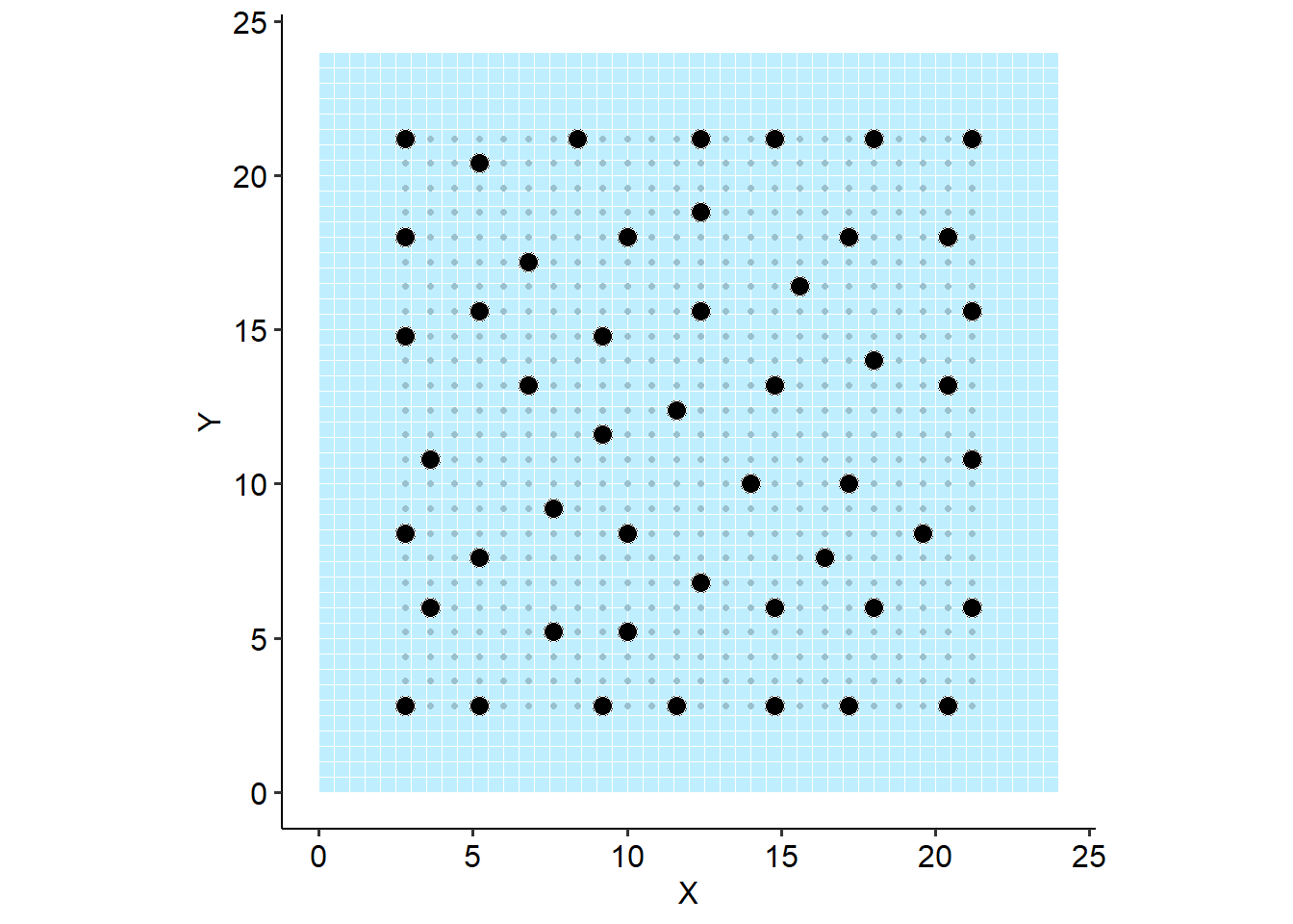
2.5 Criteria 3: constrained space-filling
Balances the \(Q_{\bar{p}}\) and \(Q_{\bar{p}_{m}}\) criteria to select for clustered “space-filling” by optimizing for the sum of probability of a capture and a movement recapture.