4 Etki Büyüklüğü Nedir?
Araştırılan ilişkinin ana kütledeki büyüklüğünü nicel olarak ifade eden ve sıfır hipotezinin ne derece yanlış olduğu anlamında tanımlanan etki büyüklüğü istatistiği, çalışma bulgularının standartlaştırılmasını sağlayarak, elde edilen değerlerin farklı değişkenler ve ölçüm yöntemleri arasında tutarlı biçimde karşılaştırılabilir ve yorumlanabilir olmasına imkân tanır (Cohen, 1988; Borenstein et al., 2009).
Meta-analizde genel olarak kullanılan etki büyüklükleri, standartlaştırılmış ortalama farkı, korelasyon ve olasılık oranıdır. Etki büyüklüğü hassasiyetini etkileyen faktörler çalışma dizaynı ve örneklem büyüklüğüdür. Tek değişkenli meta-analizde, incelenen tek değişkene ilişkin verilerin farklı araştırmacılar tarafından farklı örneklem gruplarından toplandığı kabul edilir ve tek bir etki büyüklüğü elde edilir (Kanadlı, 2021). Çok değişkenli meta-analiz ise her bir çalışmadan elde edilen birden fazla etki büyüklüğünün birleştirilmesine olanak veren yöntemdir (Cheung, 2015).
Etki büyüklüğü terimi iki değişken ya da iki grup arasındaki farkın ilişkisini nice olarak ölçmek için kullanılırken, deneysel etki kasıtlı bir uygulamanın etkisini ölçmek için kullanıldığında uygundur. Deney ve kontrol grupları arasındaki fark her iki terimle de ifade edilirken, erkek ve kadınlar arasındaki fark sadece etki büyüklüğü terimi ile ifade edilebilir (Borenstein vd., 2009).
4.1 Ortalama Farkına Dayalı Etki Büyüklükleri
Literatürde t testi deneysel ve deneysel olmayan çalışmalarda sıklıkla kullanılmaktadır. Bu çalışmalarda deney-kontrol grupları, herhangi iki grup, öntest-sontest değerleri arasındaki farklar araştırılmıştır. Bu durumda ortalama farkına dayalı etki büyüklüğü hesaplanmalıdır.
4.1.1 Standartlaştırılmamış ortalama farkı
Standartlaştırılmamış ortalama farkı, sürekli bir değişken anlamlı bir ölçekte ise ve tüm çalışmalar aynı ölçeği kullanıyorsa kullanılabilir. Farklı çalışmalar sonucu değerlendirmek için farklı araçlar (örneğin farklı psikolojik veya eğitim testleri) kullanıyorsa, ölçüm ölçeği çalışmadan çalışmaya değişir ve ham ortalama farkları birleştirmek anlamlı olmaz (Borenstein vd., 2009). Standartlaştırılmamış ortalama farkı iki grubun aritmetik ortalamalarının farkı ile hesaplanır (D). Ayrıca standart hatasının (S.H.), birleştirilmiş standart sapma değerinin (SB) ve ağırlıklandırma katsayısının (w) formülleri verilmiştir.
Standartlaştırılmamış ortalama farkının bir diğer versiyonu ise, aynı grup üzerinden elde edilen iki ölçümün karşılaştırıldığı öntest-sontest ortalamalarının farkının etki büyüklüğü değeri olarak ele alındığı durumdur. Bu fark kazanç puanı (G: gain score) şeklinde isimlendirilir ve S.H., SB ve w formülleri verilmiştir.
Formül 1. \[ \begin{align} D &= \bar{X}_{G_1} - \bar{X}_{G_2} \\ S.H. &= S_B \cdot \sqrt{\frac{1}{n_{G_1}} + \frac{1}{n_{G_2}}} \\ S_B &= \sqrt{\frac{(n_{G_1}-1)S_{G_1}^2 + (n_{G_2}-1)S_{G_2}^2}{(n_{G_1}-1) + (n_{G_2}-1)}} \\ w &= \frac{1}{(S.H.)^2} \end{align} \]
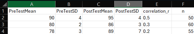
##   PreTestMean      PreTestSD    PostTestMean    PostTestSD    correlation_r
##  Min.   :78.00   Min.   :2.0   Min.   :86.0   Min.   :3.000   Min.   :0.2000
##  1st Qu.:79.00   1st Qu.:2.5   1st Qu.:87.5   1st Qu.:3.500   1st Qu.:0.2500
##  Median :80.00   Median :3.0   Median :89.0   Median :4.000   Median :0.3000
##  Mean   :82.67   Mean   :3.0   Mean   :90.0   Mean   :4.667   Mean   :0.3333
##  3rd Qu.:85.00   3rd Qu.:3.5   3rd Qu.:92.0   3rd Qu.:5.500   3rd Qu.:0.4000
##  Max.   :90.00   Max.   :4.0   Max.   :95.0   Max.   :7.000   Max.   :0.5000
##        n
##  Min.   :50.0
##  1st Qu.:52.5
##  Median :55.0
##  Mean   :55.0
##  3rd Qu.:57.5
##  Max.   :60.0
pre_test_mean <- data$PreTestMean
post_test_mean <- data$PostTestMean
pre_test_sd <- data$PreTestSD
post_test_sd <- data$PostTestSD
n <- data$n
correlation_r <- data$correlation_r
mean_diff <- post_test_mean - pre_test_mean # Ortalama farkı
mean_diff## [1] 5 6 11## [1] 4.000000 2.549510 5.385165## [1] 0.5656854 0.3894440 0.9184968## [1] 3.125000 6.593407 1.185345## [1] 5 6 11Formül 2.
\[ \begin{align} G &= \bar{X}_{T_1} - \bar{X}_{T_2} \\ S.H. &= \sqrt{\frac{2S_B^2(1-r)}{n}} \\ S_B &= \sqrt{\frac{S_{T_1}^2 + S_{T_2}^2}{2}} \\ w &= \frac{1}{(S.H.)^2} \end{align} \]
4.1.2 Standartlaştırılmış ortalama farkı
Sonuç değişkenleri karşılaştırılan iki grup eşit varyanslarla normal dağılım gösteriyorsa, standartlaştırılmış ortalama farkı, birçok istenen özelliğe sahip matematiksel olarak doğal bir etki büyüklüğü ölçüsüdür (Hedges, 2024). Standartlaştırılmış ortalama farkı (d veya g), ister aynı ister farklı ölçek kullanılsın, tüm etki büyüklüklerini ortak bir ölçü birimine dönüştürüp karşılaştırma imkânı sunar.
Cohen d, Hedges g ve Glass ∆ olmak üzere üç çeşidi vardır. d indeksi iki grubun aritmetik ortalamalarının farkının birleştirilmiş standart sapmaya bölünmesiyle elde edilir ve S.H., SB ve w formülleri verilmiştir. d indeksi 20’den küçük örneklemlerde yukarı doğru eğilimlidir (Hedges, 1981). Hedges bu formülü düzenleyip Hedges g indeksi olarak adlandırmıştır. g değeri formülü, d ve serbestlik derecesi (sd) indekslerini içermektedir. İki indeksin de S.H., SB ve w formülleri verilmiştir. Ayrıca öntest-sontest kontrol gruplu desenler için d indeksi ve S.H., SB ve w formülleri verilmiştir.
Formül 3.
Cohen d
\[ \begin{align} d &= \frac{\bar{X}_{G_1} - \bar{X}_{G_2}}{S_B} \\ S_B &= \sqrt{\frac{(n_{G_1}-1)S_{G_1}^2 + (n_{G_2}-1)S_{G_2}^2}{(n_{G_1}-1)+(n_{G_2}-1)}} \\ S.H. &= \sqrt{\frac{n_{G_1}+n_{G_2}}{n_{G_1}n_{G_2}} + \frac{d^2}{2(n_{G_1}+n_{G_2})}} \\ w &= \frac{1}{(S.H.)^2} \end{align} \]
Hedges g
\[ \begin{align} g &= \left(1 - \frac{3}{4sd - 9}\right) \cdot d \\ J &= 1 - \frac{3}{4sd - 9} \\ S.H.g &= J \cdot (S.H.d) \\ w &= \frac{1}{(S.H.g)^2} \end{align} \]
library(readxl)
# Excel dosyasını oku
data <- read_excel("s39.xlsx")
# Verilerdeki sütunları örnek olarak (değişkenler) belirleyelim
# Varsayalım ki 'pretest_mean', 'posttest_mean', 'pretest_sd', 'posttest_sd', 'n_pretest', 'n_posttest' gibi sütunlar var
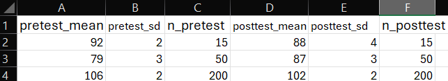
pretest_means <- data$pretest_mean
posttest_means <- data$posttest_mean
pretest_sds <- data$pretest_sd
posttest_sds <- data$posttest_sd
n_pretest <- data$n_pretest
n_posttest <- data$n_posttest
# 1. Standartlaştırılmış Etki Büyüklüğü (Cohen's d)
cohen_d <- function(M_pre, M_post, SD_pre, SD_post, n_pre, n_post) {
# Havuzlanmış standart sapmayı hesapla
SD_pooled <- sqrt(((n_pre - 1) * SD_pre^2 + (n_post - 1) * SD_post^2) / (n_pre + n_post - 2))
# Cohen's d hesapla
d <- (M_pre- M_post) / SD_pooled
return(d)
}
# 2. Cohen's d için Standart Hata (SE_d)
SE_d <- function(n_pre, n_post, d) {
SE <- sqrt((n_pre + n_post) / (n_pre * n_post) + d^2 / (2 * (n_pre + n_post)))
return(SE)
}
# 3. Hedge's g
hedges_g <- function(d, n_pre, n_post) {
g <- d * (1 - (3 / (4 * (n_pre + n_post) - 9)))
return(g)
}
# 4. Hedge's g için Standart Hata (SE_g)
SE_g <- function(SE_d, n_pre, n_post) {
SE_g <- SE_d * (1 - (3 / (4 * (n_pre + n_post) - 9)))
return(SE_g)
}
# 5. Ağırlık (W)
weight <- function(SE_d) {
w <- 1 / (SE_d^2)
return(w)
}
# Tüm makaleler için hesaplamaları yap
results <- data.frame(
study = 1:nrow(data),
d = numeric(nrow(data)),
SE_d = numeric(nrow(data)),
g = numeric(nrow(data)),
SE_g = numeric(nrow(data)),
w_d = numeric(nrow(data)),
w_g = numeric(nrow(data))
)
for(i in 1:nrow(data)) {
# Cohen's d hesapla
d_val <- cohen_d(pretest_means[i], posttest_means[i], pretest_sds[i], posttest_sds[i], n_pretest[i], n_posttest[i])
# Cohen's d için Standart Hata hesapla
SE_d_val <- SE_d(n_pretest[i], n_posttest[i], d_val)
# Hedge's g hesapla
g_val <- hedges_g(d_val, n_pretest[i], n_posttest[i])
# Hedge's g için Standart Hata hesapla
SE_g_val <- SE_g(SE_d_val, n_pretest[i], n_posttest[i])
# Ağırlık hesapla
w_d_val <- weight(SE_d_val)
w_g_val <- weight(SE_g_val)
# Sonuçları sakla
results[i, ] <- c(i, d_val, SE_d_val, g_val, SE_g_val, w_d_val, w_g_val)
}
# Sonuçları görüntüle
print(results)## study d SE_d g SE_g w_d w_g
## 1 1 1.264911 0.4000000 1.230724 0.3891892 6.25000 6.602045
## 2 2 -2.666667 0.2748737 -2.646206 0.2727647 13.23529 13.440755
## 3 3 2.000000 0.1224745 1.996229 0.1222435 66.66667 66.918794Önceki bölümlerde tek grup ön test-son test karşılaştırmasını ve iki grubun son test ortalamalarının karşılaştırılmasını içeren durumlara yer verilmiştir. Öntest-sontest kontrol gruplu deneysel desen çalışmalarında Cohen d ve Hedges g indeksleri hesaplanabilmektedir.

Formül 4.
\[ \begin{align} d &= \frac{(\bar{X}_{G_{1SON}} - \bar{X}_{G_{1ÖN}}) - (\bar{X}_{G_{2SON}} - \bar{X}_{G_{2ÖN}})}{S_B} \\ S_B &= \sqrt{\frac{(n_{G_1}-1)S_{G_{1SON}}^2 + (n_{G_2}-1)S_{G_{2SON}}^2}{(n_{G_1}-1) + (n_{G_2}-1)}} \\ S.H. &= \sqrt{\frac{n_{G_1} + n_{G_2}}{n_{G_1} n_{G_2}} + \frac{d^2}{2(n_{G_1} + n_{G_2})}} \\ w &= \frac{1}{(S.H.)^2} \end{align} \]
library(readxl)

# Excel dosyasını oku
data <- read_excel("s45.xlsx")

# Veri setinizi kontrol et
head(data)
## # A tibble: 1 × 10
## exp_pre_mean exp_post_mean control_pre_mean control_post_mean exp_pre_sd
## <dbl> <dbl> <dbl> <dbl> <dbl>
## 1 80 90 80 84 2
## # ℹ 5 more variables: exp_post_sd <dbl>, control_pre_sd <dbl>,
## # control_post_sd <dbl>, n_exp <dbl>, n_control <dbl># Verilerdeki sütunları örnek olarak (değişkenler) belirleyelim
exp_pre_mean <- data$exp_pre_mean # Deneysel grup öntest aritmetik ortalama
exp_post_mean <- data$exp_post_mean # Deneysel grup sontest aritmetik ortalama
control_pre_mean <- data$control_pre_mean # Kontrol grup öntest aritmetik ortalama
control_post_mean <- data$control_post_mean # Kontrol grup sontest aritmetik ortalama
exp_pre_sd <- data$exp_pre_sd # Deneysel grup öntest standart sapma
exp_post_sd <- data$exp_post_sd # Deneysel grup sontest standart sapma
control_pre_sd <- data$control_pre_sd # Kontrol grup öntest standart sapma
control_post_sd <- data$control_post_sd # Kontrol grup sontest standart sapma
n_exp <- data$n_exp # Deney grubu için örneklem büyüklüğü
n_control <- data$n_control # Kontrol grubu için örneklem büyüklüğü
# 1. Deneysel ve Kontrol Grubu için Cohen's d hesapla
cohen_d <- function(M_exp_pre, M_exp_post, M_control_pre, M_control_post, SD_exp_pre, SD_exp_post, SD_control_pre, SD_control_post, n_exp, n_control) {
# Havuzlanmış standart sapmayı hesapla
SD_pooled <- sqrt(((n_exp - 1) * (SD_exp_post^2) +(n_control - 1) * (SD_control_post^2)) / (n_exp + n_control - 2)) # Toplam örneklem büyüklüğü - 2
# Cohen's d hesapla: (deney post-pre) - (kontrol post-pre) / SD_pooled
d <- ((M_exp_post - M_exp_pre) - (M_control_post - M_control_pre)) / SD_pooled
return(d)
}
# 2. Standart hata (SE) hesapla
standard_error <- function(n_exp, n_control, d) {
SE <- sqrt((1 / n_exp) + (1 / n_control)+ (d^2/(2* (n_exp+ n_control))))
return(SE)
}
# 3. Ağırlık (W) hesapla: W = 1 / SE^2
weight <- function(SE) {
w <- 1 / SE^2
return(w)
}
# 4. Deneysel ve Kontrol Grubu için hesaplamaları yap
results <- data.frame(
study = 1:nrow(data),
d = numeric(nrow(data)),
w = numeric(nrow(data))
)
for(i in 1:nrow(data)) {
# Cohen's d hesapla
d_val <- cohen_d(data$exp_pre_mean[i], data$exp_post_mean[i], data$control_pre_mean[i], data$control_post_mean[i],
data$exp_pre_sd[i], data$exp_post_sd[i], data$control_pre_sd[i], data$control_post_sd[i],
data$n_exp[i], data$n_control[i])
# Havuzlanmış standart sapmayı hesapla
SD_pooled <- sqrt(((data$n_exp[i] - 1) * data$exp_pre_sd[i]^2 + (data$n_exp[i] - 1) * data$exp_post_sd[i]^2 +
(data$n_control[i] - 1) * data$control_pre_sd[i]^2 + (data$n_control[i] - 1) * data$control_post_sd[i]^2) /
(data$n_exp[i] + data$n_control[i] - 2))
# Standart hata hesapla
SE_val <- standard_error(data$n_exp[i], data$n_control[i], d_val)
# Ağırlık (W) hesapla
w_val <- weight(SE_val)
# Sonuçları sakla
results[i, ] <- c(i, d_val, w_val, SE_val)
}## Warning in matrix(value, n, p): data length [4] is not a sub-multiple or
## multiple of the number of columns [3]## study d w
## 1 1 2 33.333334.1.3 Ortalama farkına dayalı meta-analiz - örnek uygulama
Bu bölümde iki grubun ortalama farkına dayalı etki büyüklüğü değerleri kullanılarak meta analiz çalışması yapılmıştır. Bu çalışmada Hedge g, MD (standartlaştırılmamış ortalama farkı ile etki büyüklüğü), Cohen’ s d ve standart hatalar hesaplanmıştır.
library(readxl)
# Excel dosyasını oku
data <- read_excel("s176.xlsx")
# Veri setini kontrol et
head(data)## # A tibble: 6 × 6
## mean_exp sd_exp n_exp mean_control sd_control n_control
## <dbl> <dbl> <dbl> <dbl> <dbl> <dbl>
## 1 70.7 15.5 27 56.3 18.6 73
## 2 59.4 9.8 15 41.7 90.4 45
## 3 33.7 25.2 31 26.6 20.3 42
## 4 3.69 2.83 29 3.07 2.2 30
## 5 5.17 2.85 30 3.07 2.2 30
## 6 6.04 2.83 18 6.06 2.76 21# Deney ve kontrol gruplarına ait veriler
mean_exp <- data$mean_exp # Deney grubunun aritmetik ortalaması
mean_control <- data$mean_control # Kontrol grubunun aritmetik ortalaması
sd_exp <- data$sd_exp # Deney grubunun standart sapması
sd_control <- data$sd_control # Kontrol grubunun standart sapması
n_exp <- data$n_exp # Deney grubunun örneklem büyüklüğü
n_control <- data$n_control # Kontrol grubunun örneklem büyüklüğü
# 1. Birleşik Standart Sapma (Pooled Standard Deviation)
pooled_sd <- sqrt(((n_exp - 1) * sd_exp^2 + (n_control - 1) * sd_control^2) / (n_exp + n_control - 2))
# 2. Standartlaştırılmış Ortalama Fark (Cohen's d)
d <- (mean_exp - mean_control) / pooled_sd
# 3. Cohen's d için Standart Hata (SE_d)
SE_d <- sqrt((n_exp + n_control) / (n_exp * n_control) + (d^2 / (2 * (n_exp + n_control))))
# 4. Hedges's g hesaplama
g <- d * (1 - (3 / (4 * (n_exp + n_control - 2) - 1)))
# 5. Hedges's g için Standart Hata (SE_g) fonksiyonu
SE_g <- function(SE_d, n_exp, n_control) {
SE_g <- SE_d * (1 - (3 / (4 * (n_exp + n_control) - 9)))
return(SE_g)
}
SE_g_values <- SE_g(SE_d, n_exp, n_control)
# 6. Standartlaştırılmamış Ortalama Farkı (MD)
MD <- mean_exp - mean_control
# 7. MD'nin Standart Hatası (SE_MD)
SE_MD <- sqrt((sd_exp^2 / n_exp) + (sd_control^2 / n_control))
# Sonuçları yazdır
cat("Cohen's d değerleri: \n")## Cohen's d değerleri:## [1] 0.810350527 0.224885979 0.316112340 0.245140635 0.824878355
## [6] -0.007162349 1.450999155 1.644585669 0.930429782 1.264409058
## [11] 0.759959555 -1.973492204 0.145402658 -0.009238950 0.472986506
## [16] 0.577909478 -0.052614517## Cohen's d için Standart Hata değerleri:## [1] 0.2324199 0.2988484 0.2382268 0.2613912 0.2689551 0.3212091 0.2497730
## [8] 0.2701259 0.3843978 0.3999735 0.2989136 0.4608740 0.1533578 0.5000027
## [15] 0.2058997 0.2112821 0.1550166## Hedges's g değerleri:## [1] 0.804133004 0.221965382 0.312761326 0.241900890 0.814165649
## [6] -0.007016178 1.437180115 1.627394878 0.905283031 1.230235840
## [11] 0.747501202 -1.916011848 0.144756424 -0.008735008 0.469242550
## [16] 0.573185422 -0.052374997## Hedges's g için Standart Hata değerleri:## [1] 0.2306366 0.2949672 0.2357015 0.2579367 0.2654622 0.3146538 0.2473942
## [8] 0.2673023 0.3740087 0.3891635 0.2940134 0.4474505 0.1526762 0.4727298
## [15] 0.2042699 0.2095550 0.1543109## Standartlaştırılmamış Ortalama Farkı (MD) değerleri:## [1] 14.44 17.74 7.11 0.62 2.10 -0.02 18.97 23.06 1.85 1.95
## [11] 2.83 -20.72 3.75 -0.40 5.37 11.47 -0.53## MD için Standart Hata değerleri (SE_MD):## [1] 3.6946066 13.7115361 5.5007047 0.6614396 0.6573305 0.8987112
## [7] 2.9205963 3.4603797 0.7260349 0.5631400 1.0749922 3.9683075
## [13] 3.9399131 21.6474805 2.3003483 4.0235682 1.5589856# Çalışma bazında sonuçları görmek isterseniz:
results <- data.frame(
study = 1:nrow(data),
mean_exp = mean_exp,
mean_control = mean_control,
pooled_sd = pooled_sd,
d = d,
SE_d = SE_d,
g = g,
SE_g = SE_g_values,
MD = MD,
SE_MD = SE_MD
)
# Sonuçları görüntüle
print(results)
## study mean_exp mean_control pooled_sd d SE_d g
## 1 1 70.71 56.27 17.819449 0.810350527 0.2324199 0.804133004
## 2 2 59.40 41.66 78.884420 0.224885979 0.2988484 0.221965382
## 3 3 33.71 26.60 22.492004 0.316112340 0.2382268 0.312761326
## 4 4 3.69 3.07 2.529160 0.245140635 0.2613912 0.241900890
## 5 5 5.17 3.07 2.545830 0.824878355 0.2689551 0.814165649
## 6 6 6.04 6.06 2.792380 -0.007162349 0.3212091 -0.007016178
## 7 7 94.58 75.61 13.073750 1.450999155 0.2497730 1.437180115
## 8 8 98.67 75.61 14.021769 1.644585669 0.2701259 1.627394878
## 9 9 7.45 5.60 1.988328 0.930429782 0.3843978 0.905283031
## 10 10 4.40 2.45 1.542222 1.264409058 0.3999735 1.230235840
## 11 11 19.12 16.29 3.723882 0.759959555 0.2989136 0.747501202
## 12 12 45.71 66.43 10.499155 -1.973492204 0.4608740 -1.916011848
## 13 13 50.50 46.75 25.790450 0.145402658 0.1533578 0.144756424
## 14 14 52.88 53.28 43.294961 -0.009238950 0.5000027 -0.008735008
## 15 15 73.43 68.06 11.353389 0.472986506 0.2058997 0.469242550
## 16 16 55.91 44.44 19.847399 0.577909478 0.2112821 0.573185422
## 17 17 20.94 21.47 10.073266 -0.052614517 0.1550166 -0.052374997
## SE_g MD SE_MD
## 1 0.2306366 14.44 3.6946066
## 2 0.2949672 17.74 13.7115361
## 3 0.2357015 7.11 5.5007047
## 4 0.2579367 0.62 0.6614396
## 5 0.2654622 2.10 0.6573305
## 6 0.3146538 -0.02 0.8987112
## 7 0.2473942 18.97 2.9205963
## 8 0.2673023 23.06 3.4603797
## 9 0.3740087 1.85 0.7260349
## 10 0.3891635 1.95 0.5631400
## 11 0.2940134 2.83 1.0749922
## 12 0.4474505 -20.72 3.9683075
## 13 0.1526762 3.75 3.9399131
## 14 0.4727298 -0.40 21.6474805
## 15 0.2042699 5.37 2.3003483
## 16 0.2095550 11.47 4.0235682
## 17 0.1543109 -0.53 1.5589856Bu kısımda Hedge’s g, standart hata, varyans değeri, güven aralığı, z değeri ve p değeri hesaplanmıştır. Bu değerler orman garfiği kullanılarak gösterilmiştir.
library(readxl)
library(ggplot2)

# Excel dosyasını oku
data <- read_excel("s176.xlsx")

# Veri setini kontrol et
head(data)
## # A tibble: 6 × 6
## mean_exp sd_exp n_exp mean_control sd_control n_control
## <dbl> <dbl> <dbl> <dbl> <dbl> <dbl>
## 1 70.7 15.5 27 56.3 18.6 73
## 2 59.4 9.8 15 41.7 90.4 45
## 3 33.7 25.2 31 26.6 20.3 42
## 4 3.69 2.83 29 3.07 2.2 30
## 5 5.17 2.85 30 3.07 2.2 30
## 6 6.04 2.83 18 6.06 2.76 21# Deney ve kontrol gruplarına ait veriler
mean_exp <- data$mean_exp # Deney grubunun aritmetik ortalaması
mean_control <- data$mean_control # Kontrol grubunun aritmetik ortalaması
sd_exp <- data$sd_exp # Deney grubunun standart sapması
sd_control <- data$sd_control # Kontrol grubunun standart sapması
n_exp <- data$n_exp # Deney grubunun örneklem büyüklüğü
n_control <- data$n_control # Kontrol grubunun örneklem büyüklüğü
# 1. Birleşik Standart Sapma (Pooled Standard Deviation)
pooled_sd <- sqrt(((n_exp - 1) * sd_exp^2 + (n_control - 1) * sd_control^2) / (n_exp + n_control - 2))
# 2. Hedges's g hesaplama
g <- (mean_exp - mean_control) / pooled_sd * (1 - (3 / (4 * (n_exp + n_control - 2) - 1)))
# 3. Hedges's g için Standart Hata (SE_g)
SE_g <- sqrt((n_exp + n_control) / (n_exp * n_control) + (g^2 / (2 * (n_exp + n_control)))) * (1 - (3 / (4 * (n_exp + n_control) - 9)))
# 4. Varyans (Variance of g)
var_g <- SE_g^2
# 5. Güven Aralığı (95% CI)
z_critical <- 1.96 # 95% güven aralığı için
lower_ci <- g - z_critical * SE_g
upper_ci <- g + z_critical * SE_g
# 6. Z-değeri (Z-value)
z_value <- g / SE_g
# 7. P-değeri (P-value)
p_value <- 2 * (1 - pnorm(abs(z_value)))
# Sonuçları yazdır
cat("Hedges's g değerleri: \n")## Hedges's g değerleri:## [1] 0.804133004 0.221965382 0.312761326 0.241900890 0.814165649
## [6] -0.007016178 1.437180115 1.627394878 0.905283031 1.230235840
## [11] 0.747501202 -1.916011848 0.144756424 -0.008735008 0.469242550
## [16] 0.573185422 -0.052374997## Hedges's g için Standart Hata (SE_g) değerleri:## [1] 0.2305295 0.2949492 0.2356715 0.2579115 0.2651936 0.3146537 0.2469052
## [8] 0.2666053 0.3730337 0.3874314 0.2936914 0.4432254 0.1526744 0.4727295
## [15] 0.2042260 0.2094871 0.1543107## Hedges's g Varyansı (var_g):## [1] 0.05314383 0.08699506 0.05554104 0.06651832 0.07032764 0.09900697
## [7] 0.06096218 0.07107838 0.13915413 0.15010312 0.08625462 0.19644879
## [13] 0.02330948 0.22347321 0.04170828 0.04388486 0.02381179## Hedges's g için Güven Aralıkları (95% CI):## Lower Upper
## 1 0.35229528 1.2559707
## 2 -0.35613513 0.8000659
## 3 -0.14915477 0.7746774
## 4 -0.26360556 0.7474073
## 5 0.29438620 1.3339451
## 6 -0.62373750 0.6097051
## 7 0.95324593 1.9211143
## 8 1.10484852 2.1499412
## 9 0.17413700 1.6364291
## 10 0.47087022 1.9896015
## 11 0.17186613 1.3231363
## 12 -2.78473372 -1.0472900
## 13 -0.15448542 0.4439983
## 14 -0.93528488 0.9178149
## 15 0.06895951 0.8695256
## 16 0.16259063 0.9837802
## 17 -0.35482395 0.2500740## Z-değerleri (z-value):## [1] 3.48820075 0.75255451 1.32710725 0.93792224 3.07008034 -0.02229809
## [7] 5.82077712 6.10413590 2.42681307 3.17536398 2.54519301 -4.32288326
## [13] 0.94813810 -0.01847781 2.29766265 2.73613659 -0.33941263## P-değerleri (p-value):## [1] 4.862828e-04 4.517177e-01 1.844732e-01 3.482844e-01 2.140012e-03
## [6] 9.822102e-01 5.857464e-09 1.033583e-09 1.523210e-02 1.496487e-03
## [11] 1.092174e-02 1.540032e-05 3.430592e-01 9.852577e-01 2.158100e-02
## [16] 6.216522e-03 7.342989e-01# Çalışma bazında sonuçları görmek isterseniz:
results <- data.frame(
study = 1:nrow(data),
mean_exp = mean_exp,
mean_control = mean_control,
pooled_sd = pooled_sd,
g = g,
SE_g = SE_g,
var_g = var_g,
lower_ci = lower_ci,
upper_ci = upper_ci,
z_value = z_value,
p_value = p_value
)
# Sonuçları görüntüle
print(results)## study mean_exp mean_control pooled_sd g SE_g var_g
## 1 1 70.71 56.27 17.819449 0.804133004 0.2305295 0.05314383
## 2 2 59.40 41.66 78.884420 0.221965382 0.2949492 0.08699506
## 3 3 33.71 26.60 22.492004 0.312761326 0.2356715 0.05554104
## 4 4 3.69 3.07 2.529160 0.241900890 0.2579115 0.06651832
## 5 5 5.17 3.07 2.545830 0.814165649 0.2651936 0.07032764
## 6 6 6.04 6.06 2.792380 -0.007016178 0.3146537 0.09900697
## 7 7 94.58 75.61 13.073750 1.437180115 0.2469052 0.06096218
## 8 8 98.67 75.61 14.021769 1.627394878 0.2666053 0.07107838
## 9 9 7.45 5.60 1.988328 0.905283031 0.3730337 0.13915413
## 10 10 4.40 2.45 1.542222 1.230235840 0.3874314 0.15010312
## 11 11 19.12 16.29 3.723882 0.747501202 0.2936914 0.08625462
## 12 12 45.71 66.43 10.499155 -1.916011848 0.4432254 0.19644879
## 13 13 50.50 46.75 25.790450 0.144756424 0.1526744 0.02330948
## 14 14 52.88 53.28 43.294961 -0.008735008 0.4727295 0.22347321
## 15 15 73.43 68.06 11.353389 0.469242550 0.2042260 0.04170828
## 16 16 55.91 44.44 19.847399 0.573185422 0.2094871 0.04388486
## 17 17 20.94 21.47 10.073266 -0.052374997 0.1543107 0.02381179
## lower_ci upper_ci z_value p_value
## 1 0.35229528 1.2559707 3.48820075 4.862828e-04
## 2 -0.35613513 0.8000659 0.75255451 4.517177e-01
## 3 -0.14915477 0.7746774 1.32710725 1.844732e-01
## 4 -0.26360556 0.7474073 0.93792224 3.482844e-01
## 5 0.29438620 1.3339451 3.07008034 2.140012e-03
## 6 -0.62373750 0.6097051 -0.02229809 9.822102e-01
## 7 0.95324593 1.9211143 5.82077712 5.857464e-09
## 8 1.10484852 2.1499412 6.10413590 1.033583e-09
## 9 0.17413700 1.6364291 2.42681307 1.523210e-02
## 10 0.47087022 1.9896015 3.17536398 1.496487e-03
## 11 0.17186613 1.3231363 2.54519301 1.092174e-02
## 12 -2.78473372 -1.0472900 -4.32288326 1.540032e-05
## 13 -0.15448542 0.4439983 0.94813810 3.430592e-01
## 14 -0.93528488 0.9178149 -0.01847781 9.852577e-01
## 15 0.06895951 0.8695256 2.29766265 2.158100e-02
## 16 0.16259063 0.9837802 2.73613659 6.216522e-03
## 17 -0.35482395 0.2500740 -0.33941263 7.342989e-01forest_plot <- ggplot(results, aes(x = g, y = study)) +
geom_point(shape = 15, size = 3, color = "blue") + # Hedges's g noktaları
geom_errorbarh(aes(xmin = lower_ci, xmax = upper_ci), height = 0.2, color = "red") + # %95 CI yatay hata çubukları
geom_vline(xintercept = 0, linetype = "dashed", color = "black") + # 0 doğrusu
theme_minimal() +
labs(
title = "Hedges's g ve %95 Güven Aralığı Orman Grafiği",
x = "Hedges's g",
y = "Çalışma"
) +
theme(
axis.title = element_text(size = 12),
axis.text = element_text(size = 10)
) +
scale_y_continuous(
breaks = results$study,
labels = results$study
)## Warning: `geom_errobarh()` was deprecated in ggplot2 4.0.0.
## ℹ Please use the `orientation` argument of `geom_errorbar()`
## instead.
## This warning is displayed once every 8 hours.
## Call `lifecycle::last_lifecycle_warnings()` to see where this
## warning was generated.## `height` was translated to `width`.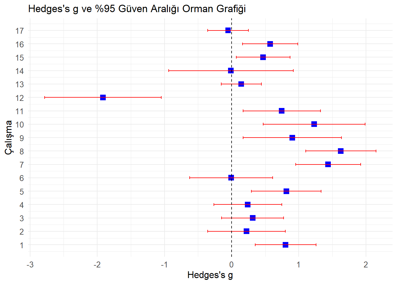
4.2 Korelasyona Dayalı Etki Büyüklüğü
Pearson çarpım-moment korelasyon katsayısı, iki değişken arasındaki kovaryansın her bir değişkenin standart sapmalarının çarpımına bölünmesi ile edilen standartlaştırılmış bir ilişki ölçüsüdür. Bu nedenle, ilişkisi incelenen değişkenler farklı şekilde ölçülse de, bir meta-analitik etki büyüklüğü istatistiği olarak kullanılabilir. Çoğu meta-analizde etki büyüklüğü, varyansın korelasyona güçlü şekilde bağlı olması nedeniyle korelasyon katsayısı ile hesaplanmaz. Korelasyonun standart formunda, korelasyon katsayısının bazı istenmeyen istatistiksel özellikleri vardır. Bu nedenle Pearson korelasyonu (r), Fisher’in z ölçeğine dönüştürülür.
Fisher’in z ile çalışırken korelasyonun varyansı kullanılmaz. Bunun yerine analizde Fisher’in z puanı ve varyansı kullanılır (Borenstein vd., 2009; Hedges & Olkin, 1985; Lipsey ve Wilson, 2001). X ve Y değişkenleri arasındaki ilişki için korelasyon katsayısı, korelasyon (r) katsayısının varyansı, Pearson korelasyon katsayısını (r) Fisher z’ye dönüştürme ve Fisher z’yi Pearson korelasyon katsayısına dönüştürme formülleri, yani sırasıyla r_xy,V_r,z,r formülleri verilmiştir.
Formül 5.
Korelasyona dayalı etki büyüklüğü
\[ \begin{align} r_{xy} &= \frac{\sigma_{xy}^2}{\sigma_x \sigma_y} \\ V_r &= \frac{(1-r^2)^2}{n-1} \end{align} \]
Fisher’s z
\[ \begin{align} z &= 0.5 \cdot \ln\left(\frac{1+r}{1-r}\right) \\ r &= \frac{e^{2z} - 1}{e^{2z} + 1} \end{align} \]
library(readxl)
# Excel dosyasını oku
data <- read_excel("s47.xlsx")
# Veri setini kontrol et
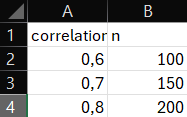
head(data)## # A tibble: 3 × 2
## correlation n
## <dbl> <dbl>
## 1 0.6 100
## 2 0.7 150
## 3 0.8 200# Verilerdeki korelasyon ve örneklem büyüklüğünü belirleyelim
r_values <- data$correlation # Korelasyon katsayıları
n_values <- data$n # Örneklem büyüklükleri
# 1. Fisher Z Dönüşümü (Korelasyonu Fisher Z'ye dönüştür)
fisher_z <- function(r) {
Z <- 0.5 * log((1 + r) / (1 - r))
return(Z)
}
# Fisher Z değerlerini hesapla
z_values <- sapply(r_values, fisher_z)
# 2. Standart hata (SE) hesaplama: SE_Z = 1 / sqrt(n - 3)
standard_error <- function(n) {
SE_Z <- 1 / sqrt(n - 3)
return(SE_Z)
}
# Standart hataları hesapla
se_values <- sapply(n_values, standard_error)
# 3. Ağırlıkları hesapla: W = 1 / SE_Z^2
weight <- function(SE_Z) {
W <- 1 / SE_Z^2
return(W)
}
# Ağırlıkları hesapla
weights <- sapply(se_values, weight)
# 4. Ağırlıklı Fisher Z hesaplama: Weighted Z = sum(W_i * Z_i) / sum(W_i)
weighted_z <- sum(weights * z_values) / sum(weights)
# 5. Ağırlıklı etki büyüklüğünü hesaplamak için Weighted Z'yi korelasyona dönüştür
r_weighted <- (exp(2 * weighted_z) - 1) / (exp(2 * weighted_z) + 1)
# Sonuçları yazdır
cat("Ağırlıklı Fisher Z değeri:", weighted_z, "\n")## Ağırlıklı Fisher Z değeri: 0.9323244## Ağırlıklı Korelasyon katsayısı (r): 0.7316758# Çalışma bazında sonuçları da görmek isterseniz:
results <- data.frame(
study = 1:nrow(data),
r = r_values,
z = z_values,
se = se_values,
weight = weights
)
# Sonuçları görüntüle
print(results)## study r z se weight
## 1 1 0.6 0.6931472 0.10153462 97
## 2 2 0.7 0.8673005 0.08247861 147
## 3 3 0.8 1.0986123 0.07124705 1974.3 Diğer Etki Büyüklükleri
İki kategorili değişkenler arasındaki ilişkilerde, deneysel uygulamalarda incelenen olayın görülme görülmeme durumunda elde edilen veriler 2x2 tablolarına aktarılıp risk oranı, olasılık oranı, risk farkları hesaplanabilir. Risk oranları için hesaplamalar logaritmik ölçekte yapılıp standart hatası hesaplanır (Borenstein vd., 2009). İki veriye dayalı etki büyüklüklerinin örneğine bu çalışmada yer verilmeyecektir.
Parametrik olmayan Veriye Dayalı Etki büyüklükleri: Normal dağılıma sahip olmayan veriler için araştırmacılar genellikle Mann–Whitney ve Wilcoxon testleri gibi parametrik olmayan istatistiksel testlere başvururlar. Bu testlerin anlamlılığı genellikle test istatistiklerinin dağılımlarının, örneklem büyüklükleri çok küçük olmadığında, z dağılımıyla değerlendirilir ve bu z değeri yardımıyla etki büyüklüğü hesaplanabilir. Örneklem büyüklüğünden bağımsız olan Cohen (1988) tarafından önerilen r=z/√N formülünden test istatistiğinden etki büyüklüğü (r) hesaplanabilir (Fritz vd., 2012). Sıra-çift serili korelasyon katsayısı gibi ölçümler parametrik ölçümlere dönüştürülürken etki büyüklüğü homojenliğini bozacağı için meta-analizde parametrik olmayan etki büyüklükleri genellikle tercih edilmemektedir.
Glass ∆: Glass’in deltası müdahale ortalamanın yanı sıra standart sapmayı da değiştirdiğinde veya iki grubun standart sapmaları arasında önemli bir fark olduğunda tercih edilebilir. Glass’ın deltasının dezavantajı, yalnızca kontrol grubunun standart sapmasını kullanmasıdır (Hedges, 1981). Bu nedenle daha küçük bir örnekleme dayanır ve daha az hassas olabilir. Belirtilen sebeplerle meta-analizde kullanılmamaktadır.
Güvenirlik genelleme ve regresyon katsayılarının meta-analizi özet olarak. ve neden ikili veriye dayalı etki büyüklüklerini ele almadığımız verilecek.