Chapter 4 Water quality

4.1 Introduction

Arsenic naturally occurs in groundwater sources around the world. Arsenic contamination of groundwater affects millions of people around the world including the United States, Nicaragua, Argentina, China, Mexico, Chile, Bangladesh, India, and Vietnam, for example (Smith et al. 2000; Amini et al. 2008; Lin et al. 2017). The World Health Organization (WHO 2018a) estimates that over 140 million people in 50 countries are exposed to arsenic contaminated drinking water above the WHO guideline of 10 \(\mu\)g/L. Health effects of arsenic exposure include numerous types of cancer and other disorders.

This project follows an analysis of a public health study performed in rural Bangladesh (Gelman et al. 2004). In this study, wells used for drinking water were analyzed for arsenic contamination and correspondingly labeled as safe or unsafe. The study determined whether households switched the well used for drinking water. Additionally, several variables where measured that were thought to possibly influence the decision of whether or not to switch wells. Here, we will investigate how accurately we can predict whether or not a household will switch wells based on these environmental variables.

4.2 Data Collection

See Gelman et al. (2004) for a discussion of data collection. Briefly, arsenic levels (in hundreds \(\mu\)g/L) were measured in Araihazar, Bangladesh during the years 1999 - 2000. Additional information was collected by a survey:

Whether or not the household switched wells.
The distance (in meters) to the closest known safe well.
Whether any members of the household are involved in community organizations.
The highest education level in the household.

4.2.1 Load necessary packages

#skimr provides a nice summary of a data set
library(skimr)
#GGally has a nice pairs plotting function
library(GGally)
#tidymodels has a nice workflow for many models. We will use it for XGBoost
library(tidymodels)
#xgboost lets us fit XGBoost models
library(xgboost)
#vip is used to visualize the importance of predicts in XGBoost models
library(vip)
#tidyverse contains packages we will use for processing and plotting data
library(tidyverse)

#Set the plotting theme
theme_set(theme_bw())

4.3 Data Preparation

4.3.1 Load the data

\(\rightarrow\) Load the data set contained in the file wells.dat and name the data frame df.

Show Coding Hint

Use read.table

Show Answer

df <- read.table("wells.dat")

4.3.2 Explore the contents of the data set

\(\rightarrow\) Look at the first few rows of the data frame.

Show Coding Hint

You can use the functions head or glimpse to see the head of the data frame or the function skim to get a nice summary.

Show Answer

head(df)

##   switch arsenic   dist assoc educ
## 1      1    2.36 16.826     0    0
## 2      1    0.71 47.322     0    0
## 3      0    2.07 20.967     0   10
## 4      1    1.15 21.486     0   12
## 5      1    1.10 40.874     1   14
## 6      1    3.90 69.518     1    9

4.3.2.1 Explore the columns

\(\rightarrow\) What are the variables?

\(\rightarrow\) What variable(s) do we want to predict?

\(\rightarrow\) What variables are possible predictors?

Show Answer

The variables in the data set are:

switch: An indicator of whether a household switches wells.
arsenic: The arsenic level of the household’s well (in hundreds \(\mu\)g/L).
dist: The distance (in meters) to the closest known safe well.
assoc: An indicator of whether any members of the household are involved in community organizations.
educ: The highest education level in the household.

We are interested in whether households switched the wells they were using after wells were labeled as either safe or unsafe, based on measured arsenic levels. So, we are trying to predict switch.

We will consider the following inputs to a model:

The distance (in meters) to the closest known safe well dist
The arsenic level of the household’s well arsenic
Whether any members of the household are involved in community organizations assoc
The highest education level in the household educ

4.3.2.2 Rename the columns

The names of the columns in this data frame are understandable, but two of the columns, switch and distance, have the names of functions that already exist in R. It is bad practice to name your variables or functions after existing functions, so we will change them. While we are at it, we will change some other names to be complete words.

df <- df %>% 
  rename(switch_well = "switch",
         distance = "dist",
         association = "assoc",
         education = "educ")

head(df)

##   switch_well arsenic distance association education
## 1           1    2.36   16.826           0         0
## 2           1    0.71   47.322           0         0
## 3           0    2.07   20.967           0        10
## 4           1    1.15   21.486           0        12
## 5           1    1.10   40.874           1        14
## 6           1    3.90   69.518           1         9

4.3.3 Further exploration of basic properties

4.3.3.1 Check for a tidy data frame

In a tidy data set, each column is a variable or id and each row is an observation.

Show Answer

Each column is a variable and each row is an observation, so the data frame is tidy. We are benefiting from some of the pre-processing that was performed on the data.

\(\rightarrow\) How many observations are in the data set? How many missing values are there in each column?

Show Answer

skim_without_charts(df)

Table 4.1: Data summary

Name	df
Number of rows	3020
Number of columns	5
_______________________
Column type frequency:
numeric	5
________________________
Group variables	None

Variable type: numeric

skim_variable	complete_rate	mean	sd	p0	p25	p50	p75	p100
switch_well	1	0.58	0.49	0.00	0.00	1.00	1.00	1.00
arsenic	1	1.66	1.11	0.51	0.82	1.30	2.20	9.65
distance	1	48.33	38.48	0.39	21.12	36.76	64.04	339.53
association	1	0.42	0.49	0.00	0.00	0.00	1.00	1.00
education	1	4.83	4.02	0.00	0.00	5.00	8.00	17.00

There are 3020 observations and no missing values.

Note that all variables are coded as numeric variables, but switch_well and association are categorical variables that happen to be coded using 0 and 1. We will convert these variables to factors.

4.3.3.2 Convert data types for qualitative predictor

\(\rightarrow\) Use the mutate function to convert switch_well and association to factors.

Show Answer

df <- df %>% 
  mutate(association = factor(association)) %>% 
  mutate(switch_well = factor(switch_well))

4.4 Exploratory data analysis

We have two main goals when doing exploratory data analysis. The first is that we want to understand the data set more completely. The second goal is to explore relationships between the variables to help guide the modeling process to answer our specific question.

4.4.1 Numerical summaries

\(\rightarrow\) What are the ranges of each of the numerical variables? Are the counts of households that switch wells and do not switch wells balanced or unbalanced? That is, do we have roughly equal numbers of households that switch wells and do not switch wells?

Show Answer

skim_without_charts(df)

Table 4.2: Data summary

Name	df
Number of rows	3020
Number of columns	5
_______________________
Column type frequency:
factor	2
numeric	3
________________________
Group variables	None

Variable type: factor

skim_variable	n_missing	complete_rate	ordered	n_unique	top_counts
switch_well	0	1	FALSE	2	1: 1737, 0: 1283
association	0	1	FALSE	2	0: 1743, 1: 1277

Variable type: numeric

skim_variable	complete_rate	mean	sd	p0	p25	p50	p75	p100
arsenic	1	1.66	1.11	0.51	0.82	1.30	2.20	9.65
distance	1	48.33	38.48	0.39	21.12	36.76	64.04	339.53
education	1	4.83	4.02	0.00	0.00	5.00	8.00	17.00

The arsenic level of the household’s well arsenic ranges from 0.51 to 9.65 (hundreds \(\mu\)g/L).

The distance (in meters) to the closest known safe well distance ranges from 0.387 to 340 meters.

The highest education level in the household education ranges from 0 to 17.

1737 of 3020 (57.5%) of households switched wells, so the counts are reasonably balanced.

4.4.2 Graphical summaries

\(\rightarrow\) Use a pairs-plot to investigate the distributions of the variables and relationships between variables. Consider the following questions:

What is the shape of the distribution of the numerical variables?
Do the predictor variables have different distributions for households that switch_well and do not switch_well wells?

Show Answer

ggpairs(df,lower = list(continuous = "cor", combo = "box_no_facet", discrete ="facetbar", na = "na"), upper = list(continuous = "points", combo ="facethist", discrete = "facetbar", na = "na"), progress = FALSE)

## `stat_bin()` using `bins = 30`. Pick better value with `binwidth`.
## `stat_bin()` using `bins = 30`. Pick better value with `binwidth`.
## `stat_bin()` using `bins = 30`. Pick better value with `binwidth`.
## `stat_bin()` using `bins = 30`. Pick better value with `binwidth`.
## `stat_bin()` using `bins = 30`. Pick better value with `binwidth`.
## `stat_bin()` using `bins = 30`. Pick better value with `binwidth`.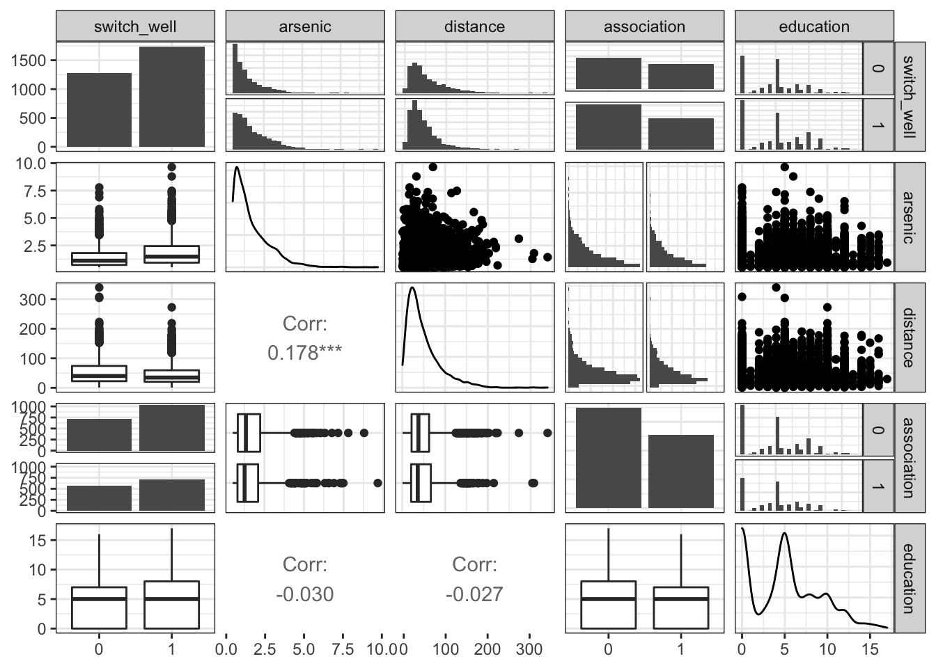

arsenic and distance have unimodal, positively skewed distributions.

education has a bimodal distribution with peaks at 0 and 5.

The distributions of arsenic, distance, and education do not appear to be obviously different for households that switch and do not switch wells.

4.4.2.1 Plot each input numerical variable vs. switch_well

We want to investigate whether the probability of switching wells is a clear function of the input numerical variables.

\(\rightarrow\) Make scatter plots of switch_well vs. each of the input numerical variables.

Show Coding Hint

Use geom_jitter so that you can see the density of points. Without jittering the points, many values lie on top of each other and it is difficult to visually estimate the probability of switching.

Show Answer

Plot switch_well vs. arsenic

df %>% 
  ggplot(aes(x = arsenic, y = switch_well)) +
  geom_jitter(width = 0, height = 0.1) +
  labs(x = "Arsenic level in nearest well", y = "Switch (No = 0, Yes = 1)")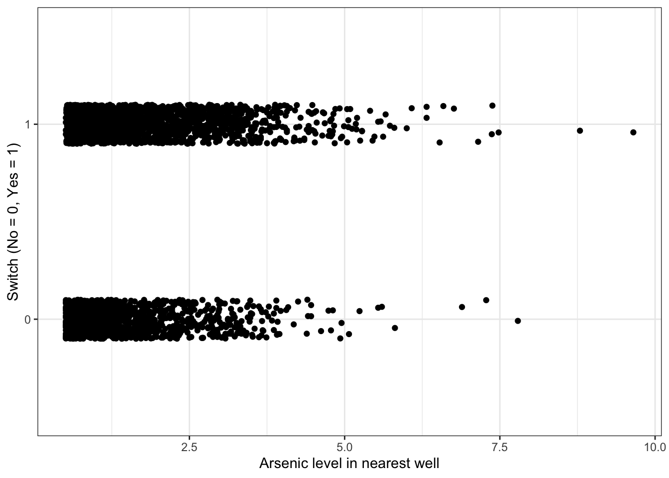

#We only add jitter in the y-direction because we don't want to change the appearance of the dependence of switching on arsenic

There appears to be a slight increase in the probability of switching as the arsenic level increases, but it is not a dramatic increase.

Plot switch_well vs. distance

df %>% 
  ggplot(aes(x = distance, y = switch_well)) +
  geom_jitter(width = 0, height = 0.1) +
  labs(x = "Distance (in meters) to the nearest safe well", y = "Switch (No = 0, Yes = 1)")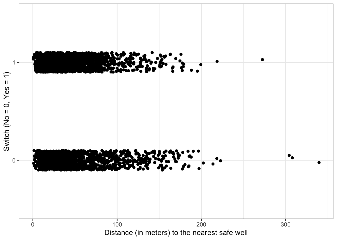

There appears to be a slight decrease in the probability of switching as distance increases, but it is not a dramatic increase.

Plot switch_well vs. education

df %>% 
  ggplot(aes(x = education, y = switch_well)) +
  geom_jitter(width = 0.15, height = 0.1) +
  labs(x = "Education level", y = "Switch (No = 0, Yes = 1)")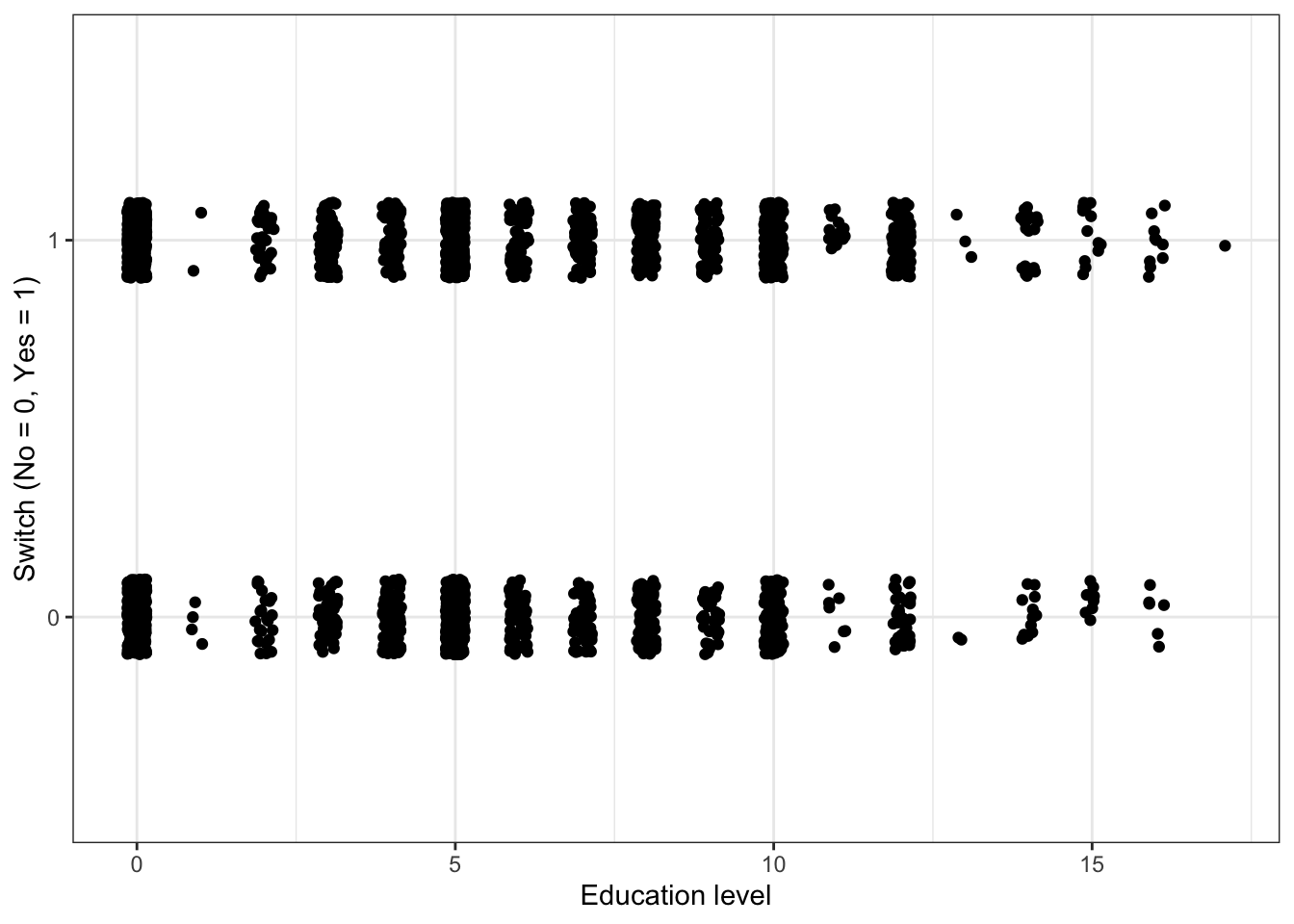

#Education is a discrete variable, so we can add jitter in the x-direction and not create any confusion.

There appears to be a slight increase in the probability of switching as the education level increases, but it is not a dramatic increase.

4.4.2.2 Examine counts of categorical variable vs. switch_well

We want to investigate whether the probability of switching wells is a clear function of the input categorical variables association.

\(\rightarrow\) Count the number of switches for each value of association. Additionally, calculate the proportion of switches for each value of association.

Show Coding Hint

Use group_by to group the data set based on association before counting the number of switches and non-switches.

Show Answer

df %>% 
  group_by(association) %>% 
  count(switch_well) %>% 
  mutate(proportion = round(n/sum(n),2)) #I like to round so that we don't see too many decimal places

## # A tibble: 4 × 4
## # Groups:   association [2]
##   association switch_well     n proportion
##   <fct>       <fct>       <int>      <dbl>
## 1 0           0             714       0.41
## 2 0           1            1029       0.59
## 3 1           0             569       0.45
## 4 1           1             708       0.55

The numbers are not hugely different, but there is a higher proportion of switches for households that are not involved in community organizations.

4.5 Exploratory modeling

We will build logistic regression models of increasing complexity in order to further understand the data.

4.5.1 Fit a model with distance as the predictor

\(\rightarrow\) Before fitting, what sign do you expect for the coefficient on distance?

Show Answer

We expect the sign of the coefficient to be negative, because it is reasonable that the probability of switching wells decreases as the distance to the nearest safe well increases.

\(\rightarrow\) Fit a logistic regression model with distance as the predictor and examine the summary.

Show Answer

Approach 1: Using glm

fit_dist <- glm(switch_well ~ distance, family=binomial, data = df)

summary(fit_dist)

## 
## Call:
## glm(formula = switch_well ~ distance, family = binomial, data = df)
## 
## Deviance Residuals: 
##     Min       1Q   Median       3Q      Max  
## -1.4406  -1.3058   0.9669   1.0308   1.6603  
## 
## Coefficients:
##               Estimate Std. Error z value Pr(>|z|)    
## (Intercept)  0.6059594  0.0603102  10.047  < 2e-16 ***
## distance    -0.0062188  0.0009743  -6.383 1.74e-10 ***
## ---
## Signif. codes:  0 '***' 0.001 '**' 0.01 '*' 0.05 '.' 0.1 ' ' 1
## 
## (Dispersion parameter for binomial family taken to be 1)
## 
##     Null deviance: 4118.1  on 3019  degrees of freedom
## Residual deviance: 4076.2  on 3018  degrees of freedom
## AIC: 4080.2
## 
## Number of Fisher Scoring iterations: 4

Approach 2: Using tidymodels

The tidymodels approach will also use glm to fit the model, but it uses a syntax that allows for a common approach to developing models of different types.

fit_dist <- logistic_reg() %>% 
  set_engine("glm") %>% 
  fit(switch_well ~ distance, data = df)

tidy(fit_dist)

## # A tibble: 2 × 5
##   term        estimate std.error statistic  p.value
##   <chr>          <dbl>     <dbl>     <dbl>    <dbl>
## 1 (Intercept)  0.606    0.0603       10.0  9.43e-24
## 2 distance    -0.00622  0.000974     -6.38 1.74e-10

It is difficult to interpret the coefficient on distance because distance is measured in meters. We don’t expect much of a change in switching behavior for wells that are 1 meter apart. A more natural measure is 100s of meters. We will scale the distance variable to be in units of 100s of meters.

\(\rightarrow\) Use the mutate function to convert the distance units into 100s of meters.

Show Answer

df <- df %>% 
  mutate(distance = distance/100)

\(\rightarrow\) Refit the model and inspect the summary. How do you expect the coefficients to change?

Show Answer

fit_dist <- logistic_reg() %>% 
  set_engine("glm") %>% 
  fit(switch_well ~ distance, data = df)

tidy(fit_dist)

## # A tibble: 2 × 5
##   term        estimate std.error statistic  p.value
##   <chr>          <dbl>     <dbl>     <dbl>    <dbl>
## 1 (Intercept)    0.606    0.0603     10.0  9.43e-24
## 2 distance      -0.622    0.0974     -6.38 1.74e-10

The intercept does not change. The coefficient on distance is multiplied by 100 from what it was before.

\(\rightarrow\) Plot the fitted logistic regression model: \[P(\text{switch_well} = 1|\text{distance}) = \frac{1}{1 + e^{-(0.61 - 0.62 \times \text{distance})}}\] along with the data.

ggplot(df,aes(x = distance, y = as.numeric(switch_well)-1)) + 
  geom_point(position = position_jitter(0,0.02)) + 
  geom_smooth(method="glm", method.args=list(family="binomial"), se=FALSE, formula = y ~ x) + 
  labs(x = "Distance (in 100 meters) to the nearest safe well", y = "Switch (No = 0, Yes = 1)")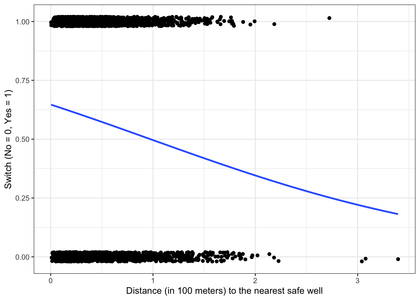

4.5.1.1 Interpret the coefficients

\(\rightarrow\) Interpret the value of \(\hat{\beta}_0\).

Show Answer

The estimated probability \[P(\text{switch_well} = 1|\text{distance} = 0) = \frac{1}{1 + e^{-\hat{\beta}_0}} = \frac{1}{1 + e^{-0.61}} = 0.65\]

The estimated probability of switching wells if the nearest safe well is where you live is 65%.

\(\rightarrow\) Interpret the value of \(\hat{\beta}_1\) by discussing its sign and what it says about the maximum rate of change of the probability of switching.

Show Answer

\(\hat{\beta}_1 < 0\), so an increase in distance to the nearest safe well is associated with a decrease in probability of switching wells.

The maximum rate of change of the probability of switching is

\[\frac{\hat{\beta}_1}{4} = \frac{-0.62}{4} = -0.155\] At the point of maximum rate of change of the probability of switching, a 100 meter increase in the distance to the nearest safe well corresponds to a decrease in probability of switching of about 16%.

4.5.2 Fit a model with distance and arsenic as predictors

Fit the model and examine the coefficients.

fit_dist_ars <- logistic_reg() %>% 
  set_engine("glm") %>% 
  fit(switch_well ~ distance + arsenic, data = df)

tidy(fit_dist_ars)

## # A tibble: 3 × 5
##   term        estimate std.error statistic  p.value
##   <chr>          <dbl>     <dbl>     <dbl>    <dbl>
## 1 (Intercept)  0.00275    0.0794    0.0346 9.72e- 1
## 2 distance    -0.897      0.104    -8.59   8.48e-18
## 3 arsenic      0.461      0.0414   11.1    8.58e-29

4.5.2.1 Explore the model

\(\rightarrow\) Interpret the meaning of the coefficients.

\(\rightarrow\) Why did the coefficient for distance change when arsenic was added?

4.5.2.2 Visualize

Plot the decision boundary

#Give a shorter name for the coefficients to make it easier to read
betas <- fit_dist_ars$fit$coefficients

df %>% 
  ggplot(aes(x = distance, y = arsenic, color = factor(switch_well))) +
  geom_point() +
  geom_abline(intercept = -betas[1]/betas[3], slope = -betas[2]/betas[3]) +
  labs(x = "Distance (in 100 meters) to the nearest safe well", y = "Arsenic concentration in well water", color = "Switch well") +
  scale_color_manual(labels = c("No", "Yes"), values = c("blue", "orange"))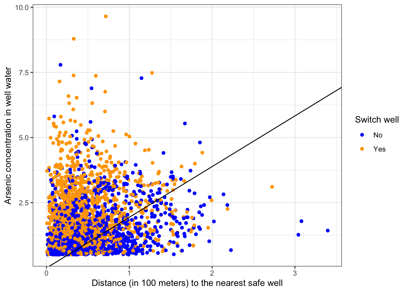

4.6 Compare models

We will use logistic regression, XGBoost, and k-nearest neighbors to construct models that predict the probability of switching wells.

To compare the different approaches, we will use a training and testing split of the data set.

We will use the tidymodels approach for all models.

4.6.1 Get train and test splits

We will split the data into training and testing sets, with 80% of the data kept for training.

#Do the split. Keep 80% for training. Use stratified sampling based on switch_well to keep the proportion of switches in the test and training sets to be approximately equal.
set.seed(12)
split <- initial_split(df, prop = 0.8, strata = switch_well)

#Extract the training and testing splits
df_train <- training(split)
df_test <- testing(split)

4.6.2 Null model

The null model prediction always predicts the value of switch_well that occurs most often in the training data.

\(\rightarrow\) What is the null model prediction for switch_well?

Show Answer

df_train %>% 
  count(switch_well)

##   switch_well    n
## 1           0 1026
## 2           1 1389

There are more households who switch in the data set, so the null model prediction is to switch wells, i.e. switch_well = 1.

If we always predict that a household will switch wells, how accurate is the prediction on test data?

null_accuracy <- sum(df_test$switch_well == 1)/length(df_test$switch_well)

null_accuracy %>% round(3)

## [1] 0.575

This represents a baseline that other models will be compared to.

4.6.3 Modeling steps using tidymodels

Using tidymodels, we will take the same steps to modeling for each type of model that we use.

Specify a model (e.g. logistic_reg(), boost_tree()) and set an engine
Create a workflow that specifies the model formula to fit and the model type
Fit any hyperparameters
Fit the model to training data
Predict using test data
Assess the model

4.6.4 Logistic regression model

4.6.4.1 Model specification

\(\rightarrow\) First specify a logistic regression model with the glm engine.

Show Answer

log_reg_model <- logistic_reg() %>%
  set_engine("glm")

4.6.4.2 Workflow

\(\rightarrow\) Create a workflow that specifies the model formula to fit and add the model specification.

Show Answer

log_reg_wf <- workflow() %>%
  add_formula(switch_well ~ .) %>%
  add_model(log_reg_model)

log_reg_wf

## ══ Workflow ═════════════════════════════════════════════════════════════════════════════════════════════════
## Preprocessor: Formula
## Model: logistic_reg()
## 
## ── Preprocessor ─────────────────────────────────────────────────────────────────────────────────────────────
## switch_well ~ .
## 
## ── Model ────────────────────────────────────────────────────────────────────────────────────────────────────
## Logistic Regression Model Specification (classification)
## 
## Computational engine: glm

4.6.4.3 Fit to training data

Fit the model to the training data and explore the coefficients.

\(\rightarrow\) First fit the model.

Show Answer

log_reg_fit <- log_reg_wf %>% 
  fit(df_train)

\(\rightarrow\) Examine the coefficients

Show Answer

tidy(log_reg_fit)

## # A tibble: 5 × 5
##   term         estimate std.error statistic  p.value
##   <chr>           <dbl>     <dbl>     <dbl>    <dbl>
## 1 (Intercept)   -0.136     0.112      -1.22 2.22e- 1
## 2 arsenic        0.428     0.0451      9.49 2.37e-21
## 3 distance      -0.898     0.117      -7.70 1.33e-14
## 4 association1  -0.113     0.0861     -1.31 1.89e- 1
## 5 education      0.0476    0.0106      4.47 7.90e- 6

In the full model, association1 and education are not statistically significant.

4.6.4.4 Predict test data

\(\rightarrow\) Generate predictions and bind the predictions together with the true switch_well values from the test data.

Show Answer

predictions_log_reg <- log_reg_fit %>%
  predict(new_data = df_test) %>% 
  bind_cols(df_test %>% select(switch_well))

Binding the predictions and actual values together into one tibble will help us to plot the confusion matrix and to compute measures of accuracy.

4.6.4.5 Assess fit

\(\rightarrow\) Plot the confusion matrix.

Show Answer

predictions_log_reg %>%
  conf_mat(switch_well, .pred_class) %>% 
  pluck(1) %>% 
  as_tibble() %>%
  ggplot(aes(Prediction, Truth, alpha = n)) +
  geom_tile(show.legend = FALSE) +
  geom_text(aes(label = n), color = "blue", alpha = 1, size = 10)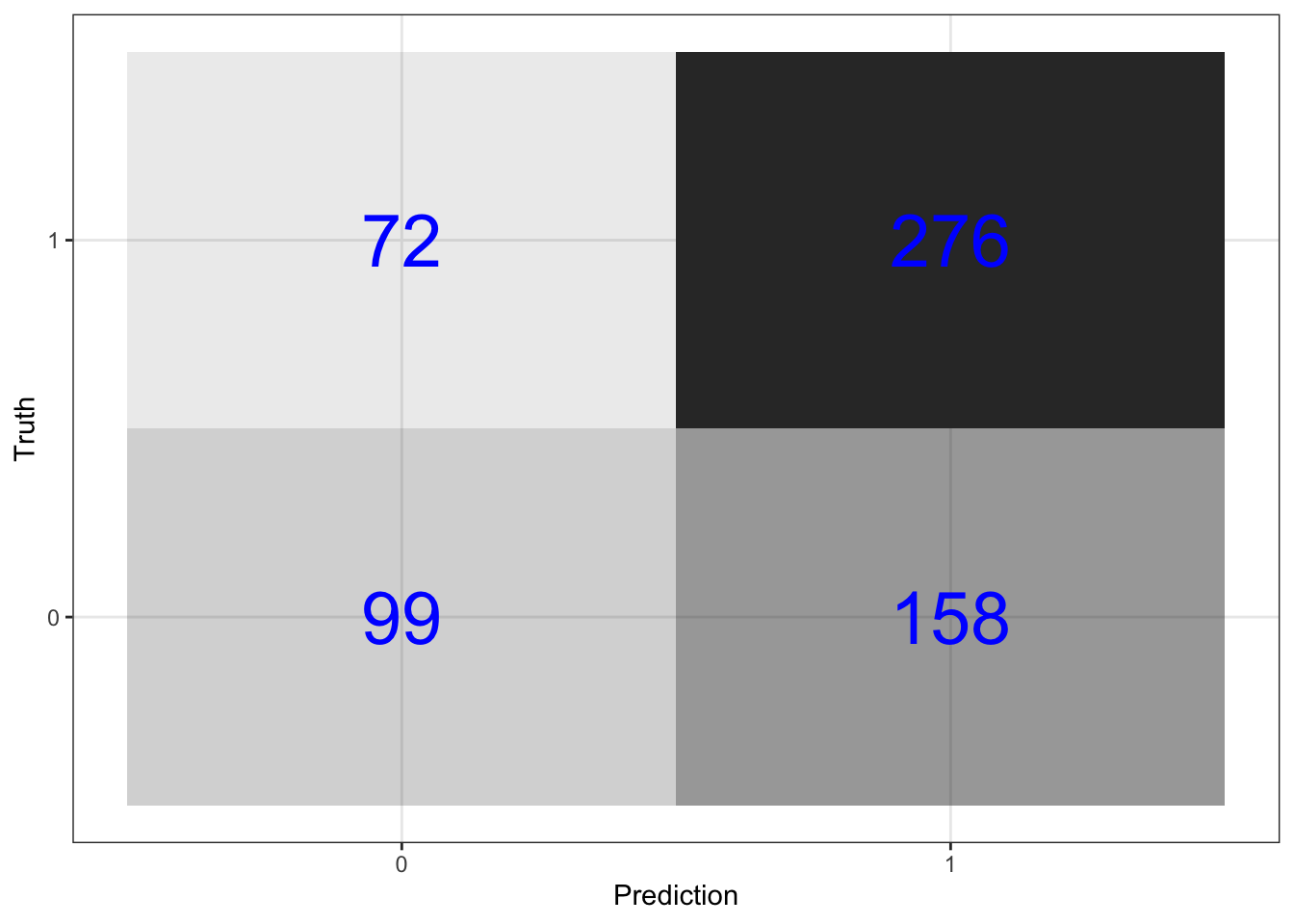

We will further analyze the performance of the model quantitatively by computing the prediction accuracy, the sensitivity, and the specificity. You should first convince yourself that you can compute these quantities by hand from the confusion matrix.

\(\rightarrow\) Get the prediction accuracy. This prediction accuracy is equal to the proportion of correct predictions in the test data set.

Show Answer

predictions_log_reg %>%
  metrics(switch_well, .pred_class) %>%
  select(-.estimator) %>%
  filter(.metric == "accuracy") %>% 
  mutate(.estimate = round(.estimate,3))

## # A tibble: 1 × 2
##   .metric  .estimate
##   <chr>        <dbl>
## 1 accuracy      0.62

\(\rightarrow\) Compare to null model prediction

Show Answer

The null model is accurate

null_accuracy %>% round(3)

## [1] 0.575

percent of the time.

\(\rightarrow\) Get the sensitivity. This is the proportion of correct predictions for households that did switch wells.

Show Answer

predictions_log_reg %>%
  sens(switch_well, .pred_class, event_level = "second") %>%
  select(-.estimator) %>%
  mutate(.estimate = round(.estimate,3))

## # A tibble: 1 × 2
##   .metric .estimate
##   <chr>       <dbl>
## 1 sens        0.793

\(\rightarrow\) Get the specificity. This is the proportion of correct predictions for households that did not switch wells.

Show Answer

predictions_log_reg %>%
  spec(switch_well, .pred_class, event_level = "second") %>%
  select(-.estimator) %>%
  mutate(.estimate = round(.estimate,3))

## # A tibble: 1 × 2
##   .metric .estimate
##   <chr>       <dbl>
## 1 spec        0.385

We are better at predicting that households will switch because there are more switches in the data set.

4.6.5 XGBoost

4.6.5.1 Set up the model

The model will be a boosted tree model, so we start by specifying the features of a boost_tree model. Theboost_tree creates a specification of a model, but does not fit the model.

\(\rightarrow\) First specify an XGBoost model for classification with the xgboost engine. Settree_depth, min_n, loss_reduction, sample_size, mtry, and learn_rate as parameters to tune. Set trees = 1000.

Show Answer

xgb_model <- boost_tree(
  mode = "classification",  #We are solving a classification problem
  trees = 1000, 
  tree_depth = tune(),  # tune() says that we will specify this parameter later
  min_n = tune(), 
  loss_reduction = tune(),                     
  sample_size = tune(), 
  mtry = tune(),         
  learn_rate = tune(),                         
  ) %>% 
  set_engine("xgboost") ## We will use xgboost to fit the model

xgb_model

## Boosted Tree Model Specification (classification)
## 
## Main Arguments:
##   mtry = tune()
##   trees = 1000
##   min_n = tune()
##   tree_depth = tune()
##   learn_rate = tune()
##   loss_reduction = tune()
##   sample_size = tune()
## 
## Computational engine: xgboost

\(\rightarrow\) Create a workflow that specifies the model formula and the model type. We are still setting up the model; this does not fit the model.

Show Answer

xgb_wf <- workflow() %>%
  add_formula(switch_well ~ .) %>%
  add_model(xgb_model)

xgb_wf

## ══ Workflow ═════════════════════════════════════════════════════════════════════════════════════════════════
## Preprocessor: Formula
## Model: boost_tree()
## 
## ── Preprocessor ─────────────────────────────────────────────────────────────────────────────────────────────
## switch_well ~ .
## 
## ── Model ────────────────────────────────────────────────────────────────────────────────────────────────────
## Boosted Tree Model Specification (classification)
## 
## Main Arguments:
##   mtry = tune()
##   trees = 1000
##   min_n = tune()
##   tree_depth = tune()
##   learn_rate = tune()
##   loss_reduction = tune()
##   sample_size = tune()
## 
## Computational engine: xgboost

4.6.5.2 Fit the model

We need to fit all of the parameters that we specified as tune().

\(\rightarrow\) Specify the parameter grid using the function grid_latin_hypercube:

Show Answer

xgb_grid <- grid_latin_hypercube(
  tree_depth(),
  min_n(),
  loss_reduction(),
  sample_size = sample_prop(),
  finalize(mtry(), df_train),
  learn_rate(),
  size = 30  #Create 30 sets of the 6 parameters
)

\(\rightarrow\) Create folds for cross-validation, using stratified sampling based on switch_well.

Show Answer

folds <- vfold_cv(df_train, strata = switch_well)

\(\rightarrow\) Do the parameter fitting.

Show Answer

xgb_grid_search <- tune_grid(
  xgb_wf,              #The workflow
  resamples = folds,   #The training data split into folds
  grid = xgb_grid,     #The grid of parameters to fit
  control = control_grid(save_pred = TRUE)
)

xgb_grid_search

## # Tuning results
## # 10-fold cross-validation using stratification 
## # A tibble: 10 × 5
##    splits             id     .metrics           .notes           .predictions         
##    <list>             <chr>  <list>             <list>           <list>               
##  1 <split [2173/242]> Fold01 <tibble [60 × 10]> <tibble [0 × 1]> <tibble [7,260 × 12]>
##  2 <split [2173/242]> Fold02 <tibble [60 × 10]> <tibble [0 × 1]> <tibble [7,260 × 12]>
##  3 <split [2173/242]> Fold03 <tibble [60 × 10]> <tibble [0 × 1]> <tibble [7,260 × 12]>
##  4 <split [2173/242]> Fold04 <tibble [60 × 10]> <tibble [0 × 1]> <tibble [7,260 × 12]>
##  5 <split [2173/242]> Fold05 <tibble [60 × 10]> <tibble [0 × 1]> <tibble [7,260 × 12]>
##  6 <split [2173/242]> Fold06 <tibble [60 × 10]> <tibble [0 × 1]> <tibble [7,260 × 12]>
##  7 <split [2174/241]> Fold07 <tibble [60 × 10]> <tibble [0 × 1]> <tibble [7,230 × 12]>
##  8 <split [2174/241]> Fold08 <tibble [60 × 10]> <tibble [0 × 1]> <tibble [7,230 × 12]>
##  9 <split [2174/241]> Fold09 <tibble [60 × 10]> <tibble [0 × 1]> <tibble [7,230 × 12]>
## 10 <split [2175/240]> Fold10 <tibble [60 × 10]> <tibble [0 × 1]> <tibble [7,200 × 12]>

\(\rightarrow\) Get the best model based on accuracy.

Show Answer

best_xgb <- select_best(xgb_grid_search, "accuracy")

\(\rightarrow\) Update the workflow with the best parameters.

Show Answer

final_xgb <- finalize_workflow(
  xgb_wf,
  best_xgb
)

final_xgb

## ══ Workflow ═════════════════════════════════════════════════════════════════════════════════════════════════
## Preprocessor: Formula
## Model: boost_tree()
## 
## ── Preprocessor ─────────────────────────────────────────────────────────────────────────────────────────────
## switch_well ~ .
## 
## ── Model ────────────────────────────────────────────────────────────────────────────────────────────────────
## Boosted Tree Model Specification (classification)
## 
## Main Arguments:
##   mtry = 3
##   trees = 1000
##   min_n = 18
##   tree_depth = 12
##   learn_rate = 0.00326302945457954
##   loss_reduction = 3.44598519830302e-08
##   sample_size = 0.871946466714144
## 
## Computational engine: xgboost

4.6.5.3 Fit to training data

\(\rightarrow\) Fit the model to the training data.

Show Answer

xgb_fit <- final_xgb %>% 
  fit(df_train)

## [17:35:03] WARNING: amalgamation/../src/learner.cc:1115: Starting in XGBoost 1.3.0, the default evaluation metric used with the objective 'binary:logistic' was changed from 'error' to 'logloss'. Explicitly set eval_metric if you'd like to restore the old behavior.

4.6.5.4 Predict test data

\(\rightarrow\) Generate predictions and bind them together with the true values from the test data.

Show Answer

predictions_xgb <- xgb_fit %>%
  predict(new_data = df_test) %>% 
  bind_cols(df_test %>% select(switch_well))

4.6.5.5 Assess fit

\(\rightarrow\) Plot the confusion matrix

Show Answer

predictions_xgb %>%
  conf_mat(switch_well, .pred_class) %>% 
  pluck(1) %>% 
  as_tibble() %>%
  ggplot(aes(Prediction, Truth, alpha = n)) +
  geom_tile(show.legend = FALSE) +
  geom_text(aes(label = n), color = "blue", alpha = 1, size = 10)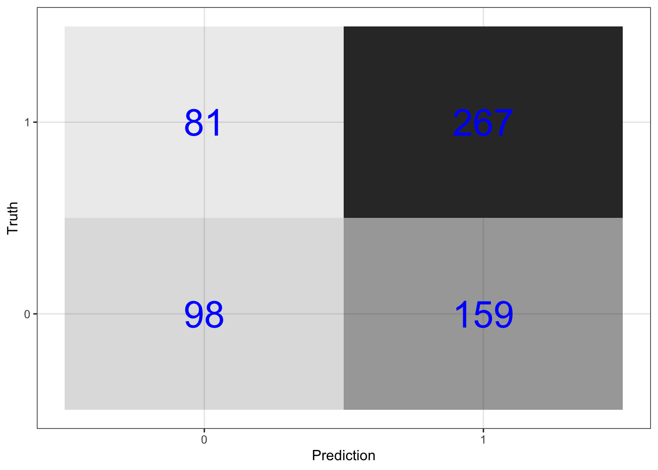

\(\rightarrow\) Get prediction accuracy. This prediction accuracy is equal to the proportion of correct predictions in the test data set.

Show Answer

predictions_xgb %>%
  metrics(switch_well, .pred_class) %>%
  select(-.estimator) %>%
  filter(.metric == "accuracy") %>% 
  mutate(.estimate = round(.estimate,3))

## # A tibble: 1 × 2
##   .metric  .estimate
##   <chr>        <dbl>
## 1 accuracy     0.603

\(\rightarrow\) Compare to null model prediction

Show Answer

The null model is accurate

null_accuracy %>% round(3)

## [1] 0.575

percent of the time.

\(\rightarrow\) Get the sensitivity. This is the proportion of correct predictions for households that did switch wells.

Show Answer

predictions_xgb %>%
  sens(switch_well, .pred_class, event_level = "second") %>%
  select(-.estimator) %>%
  mutate(.estimate = round(.estimate,3))

## # A tibble: 1 × 2
##   .metric .estimate
##   <chr>       <dbl>
## 1 sens        0.767

\(\rightarrow\) Get the specificity. This is the proportion of correct predictions for households that did not switch wells.

Show Answer

predictions_xgb %>%
  spec(switch_well, .pred_class, event_level = "second") %>%
  select(-.estimator) %>%
  mutate(.estimate = round(.estimate,3))

## # A tibble: 1 × 2
##   .metric .estimate
##   <chr>       <dbl>
## 1 spec        0.381

4.6.5.6 Relative importance of predictors

\(\rightarrow\) Look at which predictors are most important in the model

Show Answer

xgb_fit %>%
  pull_workflow_fit() %>%
  vip(geom = "col")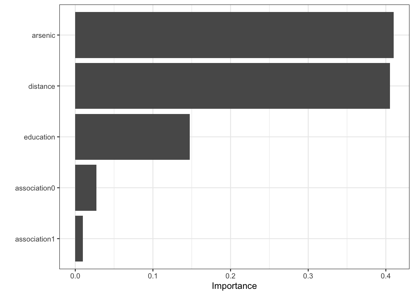

4.6.6 k nearest neighbors

4.6.6.1 Model specification

First specify a k nearest neighbors model with the knn engine.

knn_model <- nearest_neighbor(
    mode = "classification",
    neighbors = tune("K")
  ) %>%
  set_engine("kknn")

4.6.6.2 Workflow

Create a workflow that specifies the model formula to fit and the model type.

knn_wf <- workflow() %>%
  add_formula(switch_well ~ .) %>%
  add_model(knn_model)

4.6.6.3 Fit the hyperparameter k

Specify a set of values of k to try.

set.seed(1)

knn_grid <- parameters(knn_wf) %>%  
  update(K = neighbors(c(1, 50))) %>% 
  grid_latin_hypercube(size = 10)

knn_grid

## # A tibble: 10 × 1
##        K
##    <int>
##  1    40
##  2    18
##  3    49
##  4    15
##  5     7
##  6    44
##  7    29
##  8    31
##  9    22
## 10     6

Use cross validation on the previously defined folds to find the best value of k.

knn_grid_search <- tune_grid(
  knn_wf,
  resamples = folds,
  grid = knn_grid,
  control = control_grid(save_pred = TRUE)
)

knn_grid_search

## # Tuning results
## # 10-fold cross-validation using stratification 
## # A tibble: 10 × 5
##    splits             id     .metrics          .notes           .predictions        
##    <list>             <chr>  <list>            <list>           <list>              
##  1 <split [2173/242]> Fold01 <tibble [20 × 5]> <tibble [0 × 1]> <tibble [2,420 × 7]>
##  2 <split [2173/242]> Fold02 <tibble [20 × 5]> <tibble [0 × 1]> <tibble [2,420 × 7]>
##  3 <split [2173/242]> Fold03 <tibble [20 × 5]> <tibble [0 × 1]> <tibble [2,420 × 7]>
##  4 <split [2173/242]> Fold04 <tibble [20 × 5]> <tibble [0 × 1]> <tibble [2,420 × 7]>
##  5 <split [2173/242]> Fold05 <tibble [20 × 5]> <tibble [0 × 1]> <tibble [2,420 × 7]>
##  6 <split [2173/242]> Fold06 <tibble [20 × 5]> <tibble [0 × 1]> <tibble [2,420 × 7]>
##  7 <split [2174/241]> Fold07 <tibble [20 × 5]> <tibble [0 × 1]> <tibble [2,410 × 7]>
##  8 <split [2174/241]> Fold08 <tibble [20 × 5]> <tibble [0 × 1]> <tibble [2,410 × 7]>
##  9 <split [2174/241]> Fold09 <tibble [20 × 5]> <tibble [0 × 1]> <tibble [2,410 × 7]>
## 10 <split [2175/240]> Fold10 <tibble [20 × 5]> <tibble [0 × 1]> <tibble [2,400 × 7]>

Get the best model based on accuracy.

best_knn <- select_best(knn_grid_search, "accuracy")

Update the workflow with the best parameter k.

final_knn <- finalize_workflow(
  knn_wf,
  best_knn
)

final_knn

## ══ Workflow ═════════════════════════════════════════════════════════════════════════════════════════════════
## Preprocessor: Formula
## Model: nearest_neighbor()
## 
## ── Preprocessor ─────────────────────────────────────────────────────────────────────────────────────────────
## switch_well ~ .
## 
## ── Model ────────────────────────────────────────────────────────────────────────────────────────────────────
## K-Nearest Neighbor Model Specification (classification)
## 
## Main Arguments:
##   neighbors = 44
## 
## Computational engine: kknn

4.6.6.4 Fit to training data

Fit the model to the training data and explore the coefficients.

First fit the model.

set.seed(1)
knn_fit <- final_knn %>% 
  fit(df_train)

4.6.6.5 Predict test data

Generate predictions and bind together with the true values from the test data.

predictions_knn <- knn_fit %>%
  predict(new_data = df_test) %>% 
  bind_cols(df_test %>% select(switch_well))

4.6.6.6 Assess fit

Visualize the confusion matrix

predictions_knn %>%
  conf_mat(switch_well, .pred_class) %>% 
  pluck(1) %>% 
  as_tibble() %>%
  ggplot(aes(Prediction, Truth, alpha = n)) +
  geom_tile(show.legend = FALSE) +
  geom_text(aes(label = n), color = "blue", alpha = 1, size = 10)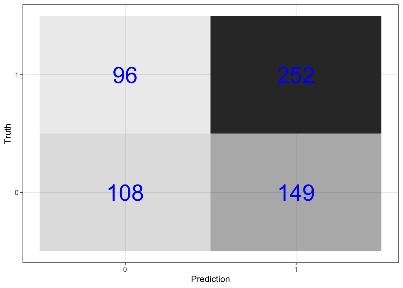

Get prediction accuracy. This prediction accuracy is equal to the proportion of correct predictions in the test data set.

predictions_knn %>%
  metrics(switch_well, .pred_class) %>%
  select(-.estimator) %>%
  filter(.metric == "accuracy") %>% 
  mutate(.estimate = round(.estimate,3))

## # A tibble: 1 × 2
##   .metric  .estimate
##   <chr>        <dbl>
## 1 accuracy     0.595

Compare to null model prediction

The null model is accurate

null_accuracy %>% round(3)

## [1] 0.575

percent of the time.

Get the sensitivity. This is the proportion of correct predictions for households that did switch wells.

predictions_knn %>%
  sens(switch_well, .pred_class, event_level = "second") %>%
  select(-.estimator) %>%
  mutate(.estimate = round(.estimate,3))

## # A tibble: 1 × 2
##   .metric .estimate
##   <chr>       <dbl>
## 1 sens        0.724

Get the specificity. This is the proportion of correct predictions for households that did not switch wells.

predictions_knn %>%
  spec(switch_well, .pred_class, event_level = "second") %>%
  select(-.estimator) %>%
  mutate(.estimate = round(.estimate,3))

## # A tibble: 1 × 2
##   .metric .estimate
##   <chr>       <dbl>
## 1 spec         0.42

4.6.7 Compare models

You used three methods to construct a model

Logistic regression
XGBoost
k nearest neighbors

Compare the performance of the models.

4.7 Additional step

Perform an additional step in the analysis of the water quality data. Consult Canvas for further directions.

4.8 Conclusion

After completing your analyses, you will make your conclusions and communicate your results. Consult Canvas for further directions.

4.1 Introduction

4.2 Data Collection

4.2.1 Load necessary packages

4.2.2 Data ethics

4.2.2.1 Data Science Ethics Checklist

4.3 Data Preparation

4.3.1 Load the data

4.3.2 Explore the contents of the data set

4.3.2.1 Explore the columns

4.3.2.2 Rename the columns

4.3.3 Further exploration of basic properties

4.3.3.1 Check for a tidy data frame

4.3.3.2 Convert data types for qualitative predictor

4.4 Exploratory data analysis

4.4.1 Numerical summaries

4.4.2 Graphical summaries

4.4.2.1 Plot each input numerical variable vs. switch_well

4.4.2.2 Examine counts of categorical variable vs. switch_well

4.5 Exploratory modeling

4.5.1 Fit a model with distance as the predictor

4.5.1.1 Interpret the coefficients

4.5.2 Fit a model with distance and arsenic as predictors

4.5.2.1 Explore the model

4.5.2.2 Visualize

4.6 Compare models

4.6.1 Get train and test splits

4.6.2 Null model

4.6.3 Modeling steps using tidymodels

4.6.4 Logistic regression model

4.6.4.1 Model specification

4.6.4.2 Workflow

4.6.4.3 Fit to training data

4.6.4.4 Predict test data

4.6.4.5 Assess fit

4.6.5 XGBoost

4.6.5.1 Set up the model

4.6.5.2 Fit the model

4.6.5.3 Fit to training data

4.6.5.4 Predict test data

4.6.5.5 Assess fit

4.6.5.6 Relative importance of predictors

4.6.6 k nearest neighbors

4.6.6.1 Model specification

4.6.6.2 Workflow

4.6.6.3 Fit the hyperparameter k

4.6.6.4 Fit to training data

4.6.6.5 Predict test data

4.6.6.6 Assess fit

4.6.7 Compare models

4.7 Additional step

4.8 Conclusion