Chapter 3 Homelessness
3.1 Introduction
The 2020 point-in-time count of people experiencing homelessness for Seattle/King County was 11,751. This represents a 5% increase over the 2019 count and reflects similar trend across many counties in the western U.S.. A step towards addressing homelessness is improving our understanding of the relationship between local housing market factors and homelessness.
The U.S. Department of Housing and Urban Development (HUD) produced a report in 2019 Market Predictors of Homelessness that describes a model-based approach to understanding of the relationship between local housing market factors and homelessness. Our project is motivated by the goals of the HUD study:
“To continue progressing toward the goals of ending and preventing homelessness, we must further our knowledge of the basic community-level determinants of homelessness. The primary objectives of this study are to (1) identify market factors that have established effects on homelessness, (2) construct and evaluate empirical models of community-level homelessness..”
We will investigate whether there are alternative modeling approaches that outperform the models described in the HUD report.
3.2 Data Collection
The data for this project are described in HUD’s report Market Predictors of Homelessness in the section titled DATA.
I will refer you to this section of the HUD report for a detailed description of the sources of the data and how they were processed.
3.2.1 Load necessary packages
#skimr provides a nice summary of a data set
library(skimr)
#leaps will be used for model selection
library(leaps)
#readxl lets us read Excel files
library(readxl)
#GGally has a nice pairs plotting function
library(GGally)
#corrplot has nice plots for correlation matrices
library(corrplot)
#gridExtra
library(gridExtra)
#glmnet is used to fit glm's. It will be used for lasso and ridge regression models.
library(glmnet)
#tidymodels has a nice workflow for many models. We will use it for XGBoost
library(tidymodels)
#xgboost lets us fit XGBoost models
library(xgboost)
#vip is used to visualize the importance of predicts in XGBoost models
library(vip)
#tidyverse contains packages we will use for processing and plotting data
library(tidyverse)

#Set the plotting theme
theme_set(theme_bw())
3.2.2 Examine the data dictionary
The data dictionary HUD TO3 - 05b Analysis File - Data Dictionary.xlsx contains descriptions of all variables in the data set.
\(\rightarrow\) Load the data dictionary (call it dictionary) and view its contents using the function View.
Show Coding Hint
Use the function read_xlsx
Show Answer
dictionary <- read_xlsx("HUD TO3 - 05b Analysis File - Data Dictionary.xlsx")View(dictionary)3.2.2.1 What are the sources of data?
\(\rightarrow\) Use the dictionary to find the unique sources of data that are not derived from other variables. We will assume that derived variables are either have Derived equal to No or Source or Root Variable starts with the string See.
Show Coding Hint
You can use the str_detect function to determine whether a string includes particular string as a component.
Show Answer
dictionary %>%
  filter(Derived == "No" & str_detect(`Source or Root Variable`, "See") == FALSE) %>%
  select(`Source or Root Variable`) %>%
  unique()
## # A tibble: 26 × 1
## `Source or Root Variable`
## <chr>
## 1 HUD
## 2 HUD PIT
## 3 HUD System Performance Measures
## 4 HUD CoC Funding Reports
## 5 HUD HIC
## 6 Census Intercensal Population Estimates
## 7 Census ACS 5-Year Estimates
## 8 Federal Housing Finance Agency
## 9 BLS Local Area Unemployment Statistics (LAUS)
## 10 Census (County Area in Sq. Miles)
## # … with 16 more rowsWhat are the sources of most of the data?
\(\rightarrow\) Make a bar graph of the counts of different data sources described in Source or Root Variable. Your graph should have the following features:
- Order the bars in descending order based on the count.
- Only include the 10 most common data sources.
- Orient the plot so that it is easy to read the labels.
Show Coding Hint
Use the fct_reorder to reorder the bars.
Use head to limit the number of bars shown.
Show Answer
dictionary %>%
  count(`Source or Root Variable`) %>%
  mutate(`Source or Root Variable` = fct_reorder(`Source or Root Variable`, n)) %>%
  head(10) %>%
  ggplot(aes(x = `Source or Root Variable`, y = n)) +
  labs(x = "Source or Root Variable", y = "Count") +
  geom_col() +
  coord_flip()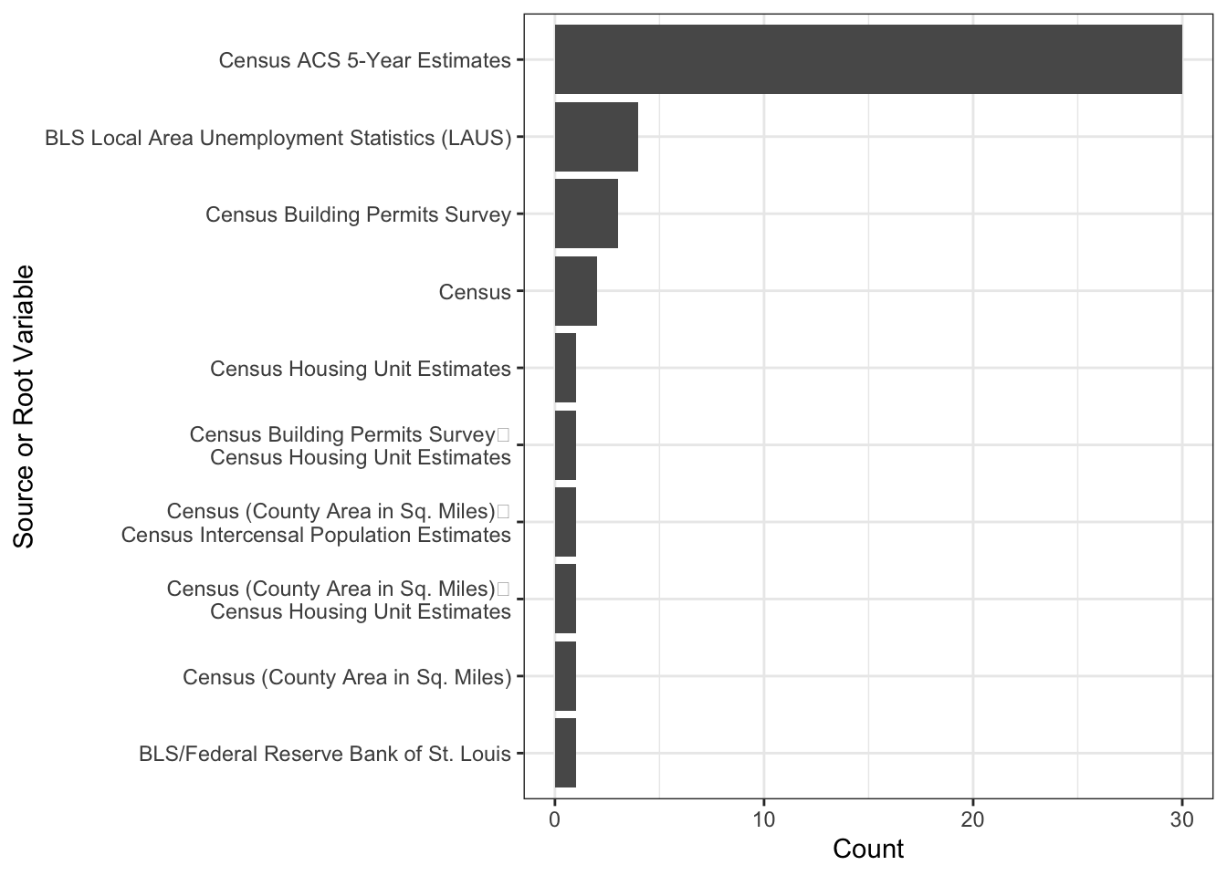
The most common source of data is the Census.
\(\rightarrow\) What are the different Associated Domains of the variables?
Show Answer
dictionary %>%
count(`Associated Domain`) %>%
mutate(`Associated Domain` = fct_reorder(`Associated Domain`, n)) %>%
ggplot(aes(x = `Associated Domain`, y = n/sum(n))) +
geom_col() +
scale_y_continuous(labels = scales::percent) +
labs(x = "Associated Domain", y = "Percentage") +
coord_flip()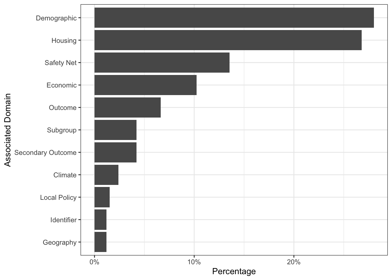 We see that there are 10 types of variables, plus an identifier. We also see that there are many demographic, housing, safety net, and economic variables. Demographic and housing variables make up more than 50% of the variables.
A big part of this project will be figuring out what variables to include in the analysis.
3.2.3 Data ethics
3.2.3.1 Data Science Ethics Checklist
![]()
A. Problem Formulation
- A.1 Well-Posed Problem: Is it possible to answer our question with data? Is the problem well-posed?
B. Data Collection
- B.1 Informed consent: If there are human subjects, have they given informed consent, where subjects affirmatively opt-in and have a clear understanding of the data uses to which they consent?
- B.2 Collection bias: Have we considered sources of bias that could be introduced during data collection and survey design and taken steps to mitigate those?
- B.3 Limit PII exposure: Have we considered ways to minimize exposure of personally identifiable information (PII) for example through anonymization or not collecting information that isn’t relevant for analysis?
- B.4 Downstream bias mitigation: Have we considered ways to enable testing downstream results for biased outcomes (e.g., collecting data on protected group status like race or gender)?
C. Data Storage
- C.1 Data security: Do we have a plan to protect and secure data (e.g., encryption at rest and in transit, access controls on internal users and third parties, access logs, and up-to-date software)?
- C.2 Right to be forgotten: Do we have a mechanism through which an individual can request their personal information be removed?
- C.3 Data retention plan: Is there a schedule or plan to delete the data after it is no longer needed?
D. Analysis
- D.1 Missing perspectives: Have we sought to address blindspots in the analysis through engagement with relevant stakeholders (e.g., checking assumptions and discussing implications with affected communities and subject matter experts)?
- D.2 Dataset bias: Have we examined the data for possible sources of bias and taken steps to mitigate or address these biases (e.g., stereotype perpetuation, confirmation bias, imbalanced classes, or omitted confounding variables)?
- D.3 Honest representation: Are our visualizations, summary statistics, and reports designed to honestly represent the underlying data?
- D.4 Privacy in analysis: Have we ensured that data with PII are not used or displayed unless necessary for the analysis?
- D.5 Auditability: Is the process of generating the analysis well documented and reproducible if we discover issues in the future?
E. Modeling
- E.1 Proxy discrimination: Have we ensured that the model does not rely on variables or proxies for variables that are unfairly discriminatory?
- E.2 Fairness across groups: Have we tested model results for fairness with respect to different affected groups (e.g., tested for disparate error rates)?
- E.3 Metric selection: Have we considered the effects of optimizing for our defined metrics and considered additional metrics?
- E.4 Explainability: Can we explain in understandable terms a decision the model made in cases where a justification is needed?
- E.5 Communicate bias: Have we communicated the shortcomings, limitations, and biases of the model to relevant stakeholders in ways that can be generally understood?
F. Deployment
- F.1 Redress: Have we discussed with our organization a plan for response if users are harmed by the results (e.g., how does the data science team evaluate these cases and update analysis and models to prevent future harm)?
- F.2 Roll back: Is there a way to turn off or roll back the model in production if necessary?
- F.3 Concept drift: Do we test and monitor for concept drift to ensure the model remains fair over time?
- F.4 Unintended use: Have we taken steps to identify and prevent unintended uses and abuse of the model and do we have a plan to monitor these once the model is deployed?
Data Science Ethics Checklist generated with deon.
We will discuss these issues in class.
3.3 Data Preparation
3.3.1 Load the data
The HUD data set is contained in the file 05b_analysis_file_update.csv.
\(\rightarrow\) Load the data set contained in the file 05b_analysis_file_update.csv and name the data frame df.
Show Coding Hint
Use read_csv
Show Answer
df <- read_csv("05b_analysis_file_update.csv")## Rows: 3008 Columns: 332
## ── Column specification ─────────────────────────────────────────────────────────────────────────────────────
## Delimiter: ","
## chr (2): cocnumber, state_abr
## dbl (329): year, pit_tot_shelt_pit_hud, pit_tot_unshelt_pit_hud, pit_tot_hless_pit_hud, pit_ind_shelt_pit...
## lgl (1): dem_health_ins_acs5yr_2012
##
## ℹ Use `spec()` to retrieve the full column specification for this data.
## ℹ Specify the column types or set `show_col_types = FALSE` to quiet this message.Note that we used read_csv, rather than read.csv because read_csv loads the data as a tibble.
3.3.2 Explore the contents of the data set
\(\rightarrow\) Look at the first few rows of the data frame.
Show Coding Hint
You can use the functions head or glimpse to see the head of the data frame or the function skim to get a nice summary.
Show Answer
head(df)## # A tibble: 6 × 332
## year cocnumber pit_tot_shelt_pit_hud pit_tot_unshelt_p… pit_tot_hless_p… pit_ind_shelt_p… pit_ind_unshelt…
## <dbl> <chr> <dbl> <dbl> <dbl> <dbl> <dbl>
## 1 2010 AK-500 1113 118 1231 633 107
## 2 2011 AK-500 1082 141 1223 677 117
## 3 2012 AK-500 1097 50 1147 756 35
## 4 2013 AK-500 1070 52 1122 792 52
## 5 2014 AK-500 970 53 1023 688 48
## 6 2015 AK-500 1029 179 1208 679 158
## # … with 325 more variables: pit_ind_hless_pit_hud <dbl>, pit_perfam_shelt_pit_hud <dbl>,
## # pit_perfam_unshelt_pit_hud <dbl>, pit_perfam_hless_pit_hud <dbl>, pit_ind_chronic_hless_pit_hud <dbl>,
## # pit_perfam_chronic_hless_pit_hud <dbl>, pit_vet_hless_pit_hud <dbl>, econ_urb_urbanicity <dbl>,
## # coctag <dbl>, panelvar <dbl>, hou_pol_totalind_hud <dbl>, hou_pol_totalday_hud <dbl>,
## # hou_pol_totalexit_hud <dbl>, hou_pol_numret6mos_hud <dbl>, hou_pol_numret12mos_hud <dbl>,
## # hou_pol_fedfundcoc <dbl>, hou_pol_fund_project <dbl>, hou_pol_bed_es_hic_hud <dbl>,
## # hou_pol_bed_oph_hic_hud <dbl>, hou_pol_bed_psh_hic_hud <dbl>, hou_pol_bed_rrh_hic_hud <dbl>, …We see that there are many columns in the data frame (332!), so it will not be easy to make sense of the data set without the data dictionary.
Refer to the data dictionary and the HUD report to understand what variables are present.
3.3.2.1 Explore the columns
What are the variables?
What variable(s) do we want to predict?
What variables seem useful as predictors?
What predictor variables are redundant?
It will take a significant amount of work to understand the contents of the data set. We will discuss this in class.
3.3.2.2 Select a subset of columns
Below are suggested variables to keep in the analysis. You may include other variables that might be useful as predictors. Provide an explanation for why you kept the variables.
\(\rightarrow\) Construct the list variable_names that we will keep for the analysis.
#Search through data dictionary to find other variables to include


variable_names <- c("year", "cocnumber",

  "pit_tot_hless_pit_hud", "pit_tot_shelt_pit_hud", "pit_tot_unshelt_pit_hud","dem_pop_pop_census",

  "fhfa_hpi_2009", "ln_hou_mkt_medrent_xt", "hou_mkt_utility_xt", "hou_mkt_burden_own_acs5yr_2017", "hou_mkt_burden_sev_rent_acs_2017", "hou_mkt_rentshare_acs5yr_2017", "hou_mkt_rentvacancy_xt", "hou_mkt_density_dummy", "hou_mkt_evict_count", "hou_mkt_ovrcrowd_acs5yr_2017", "major_city", "suburban",

           "econ_labor_unemp_rate_BLS", "econ_labor_incineq_acs5yr_2017", "econ_labor_pov_pop_census_share",

           "hou_pol_hudunit_psh_hud_share", "hou_pol_occhudunit_psh_hud", "hou_mkt_homeage1940_xt",

           "dem_soc_black_census", "dem_soc_hispanic_census", "dem_soc_asian_census", "dem_soc_pacific_census", "dem_pop_child_census", "dem_pop_senior_census", "dem_pop_female_census", "dem_pop_mig_census", "d_dem_pop_mig_census_share", "dem_soc_singadult_xt", "dem_soc_singparent_xt", "dem_soc_vet_xt", "dem_soc_ed_lessbach_xt", "dem_health_cost_dart",
           "dem_health_excesdrink_chr",

           "env_wea_avgtemp_noaa", "env_wea_avgtemp_summer_noaa", "env_wea_precip_noaa", "env_wea_precip_annual_noaa")
\(\rightarrow\) Select this subset of variables from the full data set. Call the new data frame df_small.
Coding Hint
Use the select function and your variable_names list. You should use all_of(variable_names). See https://tidyselect.r-lib.org/reference/faq-external-vector.html for an explanation of why we use all_of().
Show Answer
df_small <- df %>%
  select(all_of(variable_names))

#See https://tidyselect.r-lib.org/reference/faq-external-vector.html for an explanation of
#why we use all_of()
\(\rightarrow\) Examine the head of the new, smaller data frame.
Show Answer
head(df_small)## # A tibble: 6 × 43
## year cocnumber pit_tot_hless_pit_hud pit_tot_shelt_pit_hud pit_tot_unshelt… dem_pop_pop_cen… fhfa_hpi_2009
## <dbl> <chr> <dbl> <dbl> <dbl> <dbl> <dbl>
## 1 2010 AK-500 1231 1113 118 285194 0
## 2 2011 AK-500 1223 1082 141 293370 0.00936
## 3 2012 AK-500 1147 1097 50 296291 -0.0491
## 4 2013 AK-500 1122 1070 52 298520 -0.255
## 5 2014 AK-500 1023 970 53 301081 3.17
## 6 2015 AK-500 1208 1029 179 300296 7.33
## # … with 36 more variables: ln_hou_mkt_medrent_xt <dbl>, hou_mkt_utility_xt <dbl>,
## # hou_mkt_burden_own_acs5yr_2017 <dbl>, hou_mkt_burden_sev_rent_acs_2017 <dbl>,
## # hou_mkt_rentshare_acs5yr_2017 <dbl>, hou_mkt_rentvacancy_xt <dbl>, hou_mkt_density_dummy <dbl>,
## # hou_mkt_evict_count <dbl>, hou_mkt_ovrcrowd_acs5yr_2017 <dbl>, major_city <dbl>, suburban <dbl>,
## # econ_labor_unemp_rate_BLS <dbl>, econ_labor_incineq_acs5yr_2017 <dbl>,
## # econ_labor_pov_pop_census_share <dbl>, hou_pol_hudunit_psh_hud_share <dbl>,
## # hou_pol_occhudunit_psh_hud <dbl>, hou_mkt_homeage1940_xt <dbl>, dem_soc_black_census <dbl>, …\(\rightarrow\) Create a new dictionary for this subset of variables and use View to examine the contents.
Coding Hint
Use the filter function.
Show Answer
#Create the smaller data dictionary
dictionary_small <- dictionary %>%
  filter(Variable %in% variable_names)
#View it
dictionary_small %>%
View()How many variables of each Associated Domain are in the smaller data set?
\(\rightarrow\) Make a bar graph of the counts of different Associated Domain. Your graph should have the following features:
- Order the bars in descending order based on the count.
- Orient the plot so that it is easy to read the labels.
Show Answer
dictionary_small %>%
count(`Associated Domain`) %>%
mutate(`Associated Domain` = fct_reorder(`Associated Domain`,n)) %>%
ggplot(aes(x = `Associated Domain`, y = n)) +
geom_col() +
labs(x = "Associated Domain", y = "Count") +
coord_flip()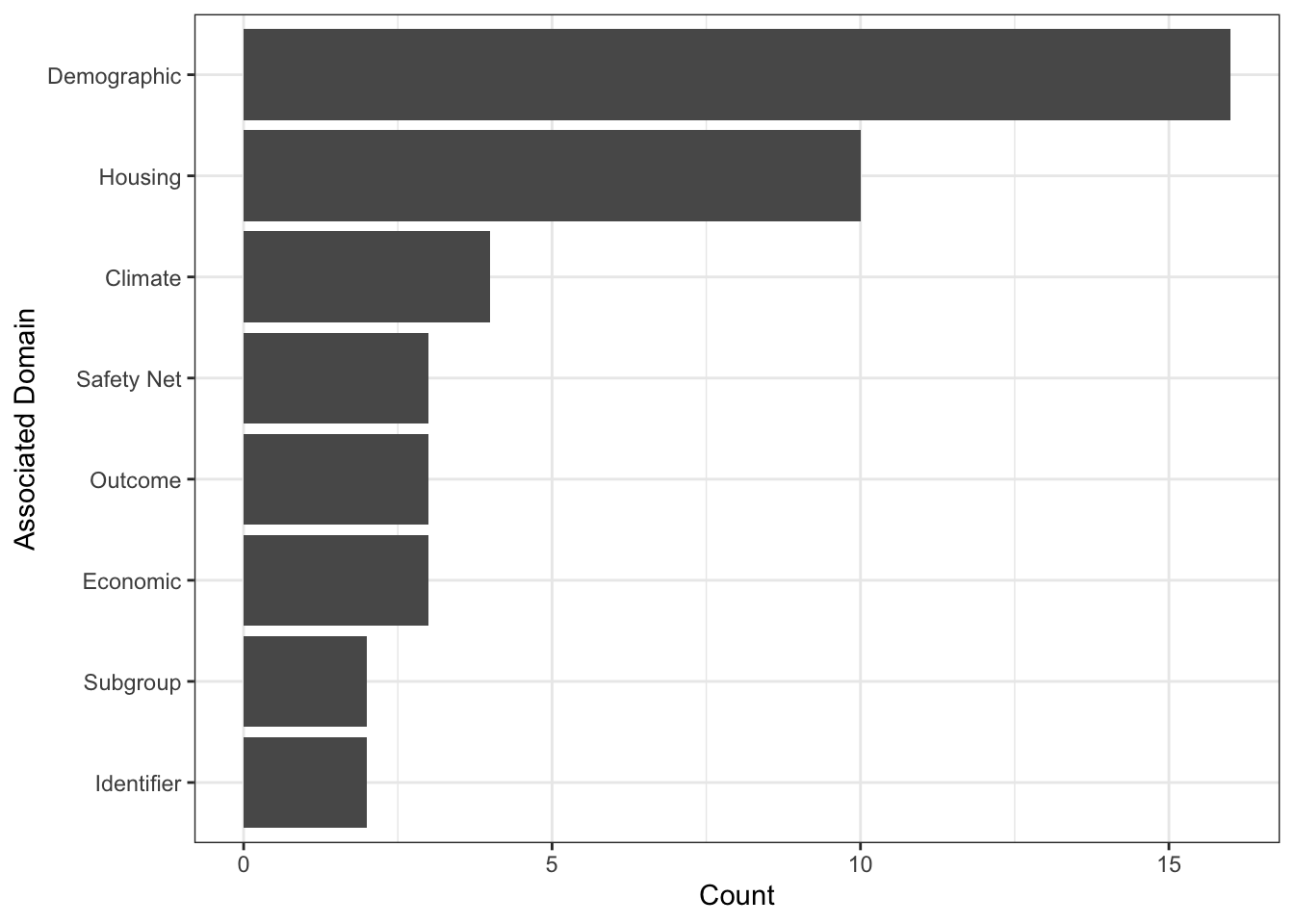 There are now 7 domains and an identifier. As with the full data frame, we have mostly demographic and housing variables.
3.3.3 Further exploration of basic properties
3.3.3.1 Check for a tidy data frame
In a tidy data set, each column is a variable or id and each row is an observation. It will take some work to determine whether the data set is tidy.
It was difficult to assess whether the full data frame was tidy because of the large number of columns with confusing names. We will do the analysis on the smaller data frame.
Show Answer
Each column is a variable or id and each row is an observation, so the data frame is tidy. We are benefiting from some of the pre-processing that HUD did with the data.
\(\rightarrow\) How many observations are in the data set?
Show Answer
nrow(df_small)## [1] 3008There are 3008 observations.
3.3.4 Data cleaning
3.3.4.1 Rename variables
I used the data dictionary to create more readable names for the minimal set of variables. You should add in new names for the additional variables you included in the data set.
The data frame with renamed columns is called df_hud.
#Add your new names to this list. If you add variable names, the order of the variables in the dictionay_small will change and you will need to reassign the numbers.

df_hud <- df_small %>%
  rename(coc_number = dictionary_small$Variable[2],
    total_sheltered = dictionary_small$Variable[3],
total_unsheltered = dictionary_small$Variable[4],
total_homeless = dictionary_small$Variable[5],
total_population = dictionary_small$Variable[6],
total_female_population = dictionary_small$Variable[7],
total_population_0_19 = dictionary_small$Variable[8],
total_population_65_plus = dictionary_small$Variable[9],
total_black = dictionary_small$Variable[10],
total_asian = dictionary_small$Variable[11],
total_pacific_islander = dictionary_small$Variable[12],
total_latino_hispanic = dictionary_small$Variable[13],
house_price_index_2009 = dictionary_small$Variable[14],
rate_unemployment = dictionary_small$Variable[15],
net_migration = dictionary_small$Variable[16],
HUD_unit_occupancy_rate = dictionary_small$Variable[17],
number_eviction = dictionary_small$Variable[18],
percentage_excessive_drinking = dictionary_small$Variable[19],
medicare_reimbursements_per_enrollee = dictionary_small$Variable[20],
average_summer_temperature = dictionary_small$Variable[21],
total_annual_precipitation = dictionary_small$Variable[22],
average_Jan_temperature = dictionary_small$Variable[23],
total_Jan_precipitation = dictionary_small$Variable[24],
gini_coefficient_2016 = dictionary_small$Variable[25],
poverty_rate = dictionary_small$Variable[26],
share_renters_2016 = dictionary_small$Variable[27],
share_overcrowded_units_2016 = dictionary_small$Variable[28],
percentage_owners_cost_burden_2016 = dictionary_small$Variable[29],
percentage_renters_severe_cost_burden_2016 = dictionary_small$Variable[30],
share_HUD_units = dictionary_small$Variable[31],
high_housing_density = dictionary_small$Variable[32],
share_built_before_1940  = dictionary_small$Variable[33],
utility_costs  = dictionary_small$Variable[34],
rental_vacancy_rate = dictionary_small$Variable[35],
proportion_one_person_households  = dictionary_small$Variable[36],
share_under_18_with_single_parent = dictionary_small$Variable[37],
share_veteran_status = dictionary_small$Variable[38],
log_median_rent = dictionary_small$Variable[39],
migration_4_year_change  = dictionary_small$Variable[40],
share_no_bachelors = dictionary_small$Variable[41],
city_or_urban = dictionary_small$Variable[42],
suburban = dictionary_small$Variable[43]
)
\(\rightarrow\) Examine the head of the new data frame with the updated names:
Show Answer
head(df_hud)## # A tibble: 6 × 43
## year coc_number total_homeless total_sheltered total_unsheltered total_population house_price_index_2009
## <dbl> <chr> <dbl> <dbl> <dbl> <dbl> <dbl>
## 1 2010 AK-500 1231 1113 118 285194 0
## 2 2011 AK-500 1223 1082 141 293370 0.00936
## 3 2012 AK-500 1147 1097 50 296291 -0.0491
## 4 2013 AK-500 1122 1070 52 298520 -0.255
## 5 2014 AK-500 1023 970 53 301081 3.17
## 6 2015 AK-500 1208 1029 179 300296 7.33
## # … with 36 more variables: log_median_rent <dbl>, utility_costs <dbl>,
## # percentage_owners_cost_burden_2016 <dbl>, percentage_renters_severe_cost_burden_2016 <dbl>,
## # share_renters_2016 <dbl>, rental_vacancy_rate <dbl>, high_housing_density <dbl>, number_eviction <dbl>,
## # share_overcrowded_units_2016 <dbl>, city_or_urban <dbl>, suburban <dbl>, rate_unemployment <dbl>,
## # gini_coefficient_2016 <dbl>, poverty_rate <dbl>, share_HUD_units <dbl>, HUD_unit_occupancy_rate <dbl>,
## # share_built_before_1940 <dbl>, total_black <dbl>, total_latino_hispanic <dbl>, total_asian <dbl>,
## # total_pacific_islander <dbl>, total_population_0_19 <dbl>, total_population_65_plus <dbl>, …\(\rightarrow\) Display the names of the columns of the new data frame:
Show Answer
names(df_hud)## [1] "year" "coc_number"
## [3] "total_homeless" "total_sheltered"
## [5] "total_unsheltered" "total_population"
## [7] "house_price_index_2009" "log_median_rent"
## [9] "utility_costs" "percentage_owners_cost_burden_2016"
## [11] "percentage_renters_severe_cost_burden_2016" "share_renters_2016"
## [13] "rental_vacancy_rate" "high_housing_density"
## [15] "number_eviction" "share_overcrowded_units_2016"
## [17] "city_or_urban" "suburban"
## [19] "rate_unemployment" "gini_coefficient_2016"
## [21] "poverty_rate" "share_HUD_units"
## [23] "HUD_unit_occupancy_rate" "share_built_before_1940"
## [25] "total_black" "total_latino_hispanic"
## [27] "total_asian" "total_pacific_islander"
## [29] "total_population_0_19" "total_population_65_plus"
## [31] "total_female_population" "net_migration"
## [33] "migration_4_year_change" "proportion_one_person_households"
## [35] "share_under_18_with_single_parent" "share_veteran_status"
## [37] "share_no_bachelors" "medicare_reimbursements_per_enrollee"
## [39] "percentage_excessive_drinking" "average_Jan_temperature"
## [41] "average_summer_temperature" "total_Jan_precipitation"
## [43] "total_annual_precipitation"Renaming the variables is a huge pain, but I find that it helps me to understand what the variables represent. This is useful for projects where you will spend a significant amount of time with the data.
3.3.5 Identify and deal with missing values
\(\rightarrow\) How many missing values are there in each column? Give the number of missing values and the percent of values in each column that are missing.
Show Coding Hing
The skim function shows the number of missing values and the completion rate for each column. You can also use skim_without_charts to get the same information without the graphs.
Show Answer
Recall that missing values may be coded with NA, or they may be empty. We want to convert empty cells to NA, so that we can use the function is.na to find all missing values. The function read_csv that we used to read in the data does this automatically, so we do not need to take further action to deal with empty cells. Note that the default argument in read_csv that controls this is na = c("", "NA"), which means that empty cells or NA values are treated as NA.
skim_without_charts(df_hud)| Name | df_hud |
| Number of rows | 3008 |
| Number of columns | 43 |
| _______________________ | |
| Column type frequency: | |
| character | 1 |
| numeric | 42 |
| ________________________ | |
| Group variables | None |
Variable type: character
| skim_variable | n_missing | complete_rate | min | max | empty | n_unique | whitespace |
|---|---|---|---|---|---|---|---|
| coc_number | 0 | 1 | 6 | 7 | 0 | 376 | 0 |
Variable type: numeric
| skim_variable | n_missing | complete_rate | mean | sd | p0 | p25 | p50 | p75 | p100 |
|---|---|---|---|---|---|---|---|---|---|
| year | 0 | 1.00 | 2013.50 | 2.29 | 2010.00 | 2011.75 | 2013.50 | 2015.25 | 2017.00 |
| total_homeless | 14 | 1.00 | 1560.43 | 4313.39 | 7.00 | 320.25 | 679.00 | 1468.00 | 76501.00 |
| total_sheltered | 14 | 1.00 | 1033.85 | 3445.81 | 3.00 | 224.00 | 445.50 | 961.50 | 72565.00 |
| total_unsheltered | 14 | 1.00 | 526.58 | 1742.31 | 0.00 | 36.25 | 114.00 | 418.25 | 42828.00 |
| total_population | 0 | 1.00 | 837457.01 | 1217309.59 | 29344.00 | 266710.75 | 481798.50 | 896909.25 | 11058958.00 |
| house_price_index_2009 | 0 | 1.00 | -2.74 | 10.14 | -26.50 | -8.61 | -3.28 | 0.00 | 63.86 |
| log_median_rent | 1504 | 0.50 | 1.97 | 0.31 | 1.24 | 1.73 | 1.94 | 2.16 | 2.87 |
| utility_costs | 1504 | 0.50 | 14.66 | 3.10 | 5.60 | 12.60 | 14.80 | 16.90 | 22.60 |
| percentage_owners_cost_burden_2016 | 0 | 1.00 | 14.87 | 3.04 | 8.07 | 12.48 | 14.39 | 17.08 | 22.96 |
| percentage_renters_severe_cost_burden_2016 | 0 | 1.00 | 25.54 | 3.86 | 16.38 | 22.86 | 25.00 | 27.76 | 37.65 |
| share_renters_2016 | 0 | 1.00 | 34.55 | 8.23 | 15.10 | 28.64 | 33.52 | 39.66 | 69.22 |
| rental_vacancy_rate | 1504 | 0.50 | 7.15 | 2.98 | 1.92 | 5.20 | 6.60 | 8.40 | 24.63 |
| high_housing_density | 0 | 1.00 | 0.25 | 0.43 | 0.00 | 0.00 | 0.00 | 0.25 | 1.00 |
| number_eviction | 0 | 1.00 | 2501.98 | 4314.93 | 0.00 | 96.75 | 935.50 | 2693.00 | 37105.00 |
| share_overcrowded_units_2016 | 0 | 1.00 | 2.70 | 1.95 | 0.66 | 1.51 | 2.04 | 3.04 | 12.26 |
| city_or_urban | 0 | 1.00 | 0.28 | 0.45 | 0.00 | 0.00 | 0.00 | 1.00 | 1.00 |
| suburban | 0 | 1.00 | 0.43 | 0.49 | 0.00 | 0.00 | 0.00 | 1.00 | 1.00 |
| rate_unemployment | 0 | 1.00 | 7.48 | 2.70 | 2.51 | 5.51 | 7.18 | 8.94 | 28.86 |
| gini_coefficient_2016 | 0 | 1.00 | 45.52 | 2.85 | 37.56 | 43.70 | 45.40 | 46.99 | 54.78 |
| poverty_rate | 0 | 1.00 | 14.42 | 4.46 | 3.35 | 11.45 | 14.32 | 17.31 | 35.79 |
| share_HUD_units | 0 | 1.00 | 3.65 | 1.92 | 0.09 | 2.32 | 3.30 | 4.69 | 13.96 |
| HUD_unit_occupancy_rate | 0 | 1.00 | 92.60 | 3.99 | 69.44 | 90.77 | 93.01 | 95.15 | 100.00 |
| share_built_before_1940 | 1504 | 0.50 | 13.46 | 10.78 | 0.22 | 4.88 | 10.11 | 20.13 | 56.88 |
| total_black | 0 | 1.00 | 103606.65 | 202325.49 | 152.00 | 10567.00 | 36742.00 | 109931.25 | 1956449.00 |
| total_latino_hispanic | 0 | 1.00 | 142104.15 | 407635.29 | 224.00 | 14898.50 | 35744.50 | 92569.50 | 4924272.00 |
| total_asian | 0 | 1.00 | 42375.38 | 117157.23 | 80.00 | 4291.75 | 11239.50 | 30542.50 | 1474987.00 |
| total_pacific_islander | 0 | 1.00 | 1388.47 | 5558.70 | 1.00 | 117.00 | 259.00 | 642.25 | 89016.00 |
| total_population_0_19 | 0 | 1.00 | 219436.13 | 329651.86 | 6194.00 | 67781.25 | 124462.00 | 234535.00 | 3204024.00 |
| total_population_65_plus | 0 | 1.00 | 117131.31 | 161665.55 | 4781.00 | 38146.75 | 66976.00 | 124377.25 | 1525916.00 |
| total_female_population | 0 | 1.00 | 425237.98 | 618118.92 | 14816.00 | 135979.25 | 244430.50 | 461586.00 | 5542088.00 |
| net_migration | 0 | 1.00 | 2458.73 | 8426.78 | -41321.00 | -719.00 | 492.50 | 3207.75 | 101369.00 |
| migration_4_year_change | 2632 | 0.12 | 0.07 | 0.68 | -3.45 | -0.26 | 0.02 | 0.36 | 2.60 |
| proportion_one_person_households | 1504 | 0.50 | 27.73 | 4.15 | 12.48 | 25.40 | 27.82 | 30.10 | 46.71 |
| share_under_18_with_single_parent | 1504 | 0.50 | 25.58 | 6.94 | 9.44 | 20.94 | 24.61 | 29.21 | 55.63 |
| share_veteran_status | 1504 | 0.50 | 10.89 | 3.05 | 2.80 | 8.96 | 10.78 | 12.66 | 23.88 |
| share_no_bachelors | 1504 | 0.50 | 69.69 | 10.30 | 23.69 | 64.34 | 71.09 | 77.36 | 88.64 |
| medicare_reimbursements_per_enrollee | 0 | 1.00 | 9.36 | 1.25 | 6.03 | 8.44 | 9.22 | 10.08 | 17.95 |
| percentage_excessive_drinking | 2632 | 0.12 | 0.19 | 0.03 | 0.11 | 0.17 | 0.19 | 0.21 | 0.29 |
| average_Jan_temperature | 0 | 1.00 | 35.36 | 12.85 | -3.24 | 26.32 | 33.71 | 44.11 | 74.70 |
| average_summer_temperature | 2 | 1.00 | 74.05 | 6.17 | 55.80 | 69.54 | 73.90 | 78.74 | 93.25 |
| total_Jan_precipitation | 0 | 1.00 | 2.94 | 2.51 | 0.00 | 1.33 | 2.53 | 3.59 | 25.32 |
| total_annual_precipitation | 0 | 1.00 | 41.03 | 15.36 | 1.25 | 33.52 | 42.03 | 49.96 | 105.19 |
Most variables are not missing any values, but there are many variables that are missing half or more of the values.
We are interested in predicting the number of people experiencing homelessness. So, we will remove the rows where those numbers are missing.
\(\rightarrow\) Remove the rows where total_homeless is NA.
Show Coding Hint
Use the filter function.
Show Answer
df_hud <- df_hud %>%
filter(is.na(total_homeless) == FALSE)skim_without_charts(df_hud)| Name | df_hud |
| Number of rows | 2994 |
| Number of columns | 43 |
| _______________________ | |
| Column type frequency: | |
| character | 1 |
| numeric | 42 |
| ________________________ | |
| Group variables | None |
Variable type: character
| skim_variable | n_missing | complete_rate | min | max | empty | n_unique | whitespace |
|---|---|---|---|---|---|---|---|
| coc_number | 0 | 1 | 6 | 7 | 0 | 376 | 0 |
Variable type: numeric
| skim_variable | n_missing | complete_rate | mean | sd | p0 | p25 | p50 | p75 | p100 |
|---|---|---|---|---|---|---|---|---|---|
| year | 0 | 1.00 | 2013.50 | 2.29 | 2010.00 | 2012.00 | 2013.00 | 2015.00 | 2017.00 |
| total_homeless | 0 | 1.00 | 1560.43 | 4313.39 | 7.00 | 320.25 | 679.00 | 1468.00 | 76501.00 |
| total_sheltered | 0 | 1.00 | 1033.85 | 3445.81 | 3.00 | 224.00 | 445.50 | 961.50 | 72565.00 |
| total_unsheltered | 0 | 1.00 | 526.58 | 1742.31 | 0.00 | 36.25 | 114.00 | 418.25 | 42828.00 |
| total_population | 0 | 1.00 | 840371.32 | 1219259.79 | 29344.00 | 267388.75 | 484041.50 | 900588.25 | 11058958.00 |
| house_price_index_2009 | 0 | 1.00 | -2.72 | 10.15 | -26.50 | -8.60 | -3.25 | 0.00 | 63.86 |
| log_median_rent | 1495 | 0.50 | 1.97 | 0.31 | 1.24 | 1.73 | 1.94 | 2.16 | 2.87 |
| utility_costs | 1495 | 0.50 | 14.65 | 3.11 | 5.60 | 12.60 | 14.80 | 16.90 | 22.60 |
| percentage_owners_cost_burden_2016 | 0 | 1.00 | 14.87 | 3.04 | 8.07 | 12.48 | 14.39 | 17.07 | 22.96 |
| percentage_renters_severe_cost_burden_2016 | 0 | 1.00 | 25.56 | 3.84 | 16.38 | 22.86 | 25.00 | 27.85 | 37.65 |
| share_renters_2016 | 0 | 1.00 | 34.55 | 8.25 | 15.10 | 28.55 | 33.53 | 39.73 | 69.22 |
| rental_vacancy_rate | 1495 | 0.50 | 7.14 | 2.98 | 1.92 | 5.20 | 6.59 | 8.40 | 24.63 |
| high_housing_density | 0 | 1.00 | 0.25 | 0.43 | 0.00 | 0.00 | 0.00 | 1.00 | 1.00 |
| number_eviction | 0 | 1.00 | 2513.26 | 4321.83 | 0.00 | 107.50 | 941.50 | 2722.00 | 37105.00 |
| share_overcrowded_units_2016 | 0 | 1.00 | 2.71 | 1.95 | 0.66 | 1.51 | 2.05 | 3.06 | 12.26 |
| city_or_urban | 0 | 1.00 | 0.28 | 0.45 | 0.00 | 0.00 | 0.00 | 1.00 | 1.00 |
| suburban | 0 | 1.00 | 0.43 | 0.49 | 0.00 | 0.00 | 0.00 | 1.00 | 1.00 |
| rate_unemployment | 0 | 1.00 | 7.48 | 2.71 | 2.51 | 5.50 | 7.18 | 8.94 | 28.86 |
| gini_coefficient_2016 | 0 | 1.00 | 45.53 | 2.85 | 37.56 | 43.70 | 45.42 | 47.01 | 54.78 |
| poverty_rate | 0 | 1.00 | 14.42 | 4.47 | 3.35 | 11.43 | 14.32 | 17.31 | 35.79 |
| share_HUD_units | 0 | 1.00 | 3.66 | 1.91 | 0.09 | 2.32 | 3.29 | 4.70 | 13.96 |
| HUD_unit_occupancy_rate | 0 | 1.00 | 92.60 | 3.99 | 69.44 | 90.77 | 93.01 | 95.15 | 100.00 |
| share_built_before_1940 | 1495 | 0.50 | 13.44 | 10.76 | 0.22 | 4.88 | 10.13 | 20.12 | 56.88 |
| total_black | 0 | 1.00 | 104005.74 | 202698.30 | 168.00 | 10750.00 | 36833.00 | 110397.25 | 1956449.00 |
| total_latino_hispanic | 0 | 1.00 | 142706.42 | 408490.87 | 224.00 | 15101.25 | 36013.00 | 93348.75 | 4924272.00 |
| total_asian | 0 | 1.00 | 42564.47 | 117398.02 | 80.00 | 4369.00 | 11316.50 | 30792.50 | 1474987.00 |
| total_pacific_islander | 0 | 1.00 | 1394.53 | 5570.97 | 1.00 | 117.00 | 259.50 | 646.50 | 89016.00 |
| total_population_0_19 | 0 | 1.00 | 220205.33 | 330188.04 | 6194.00 | 67984.75 | 124752.50 | 235074.50 | 3204024.00 |
| total_population_65_plus | 0 | 1.00 | 117515.06 | 161921.65 | 5132.00 | 38351.75 | 67198.50 | 124875.25 | 1525916.00 |
| total_female_population | 0 | 1.00 | 426719.90 | 619107.26 | 14816.00 | 136479.75 | 246606.00 | 464249.50 | 5542088.00 |
| net_migration | 0 | 1.00 | 2470.68 | 8444.32 | -41321.00 | -720.50 | 501.50 | 3211.50 | 101369.00 |
| migration_4_year_change | 2620 | 0.12 | 0.07 | 0.68 | -3.45 | -0.26 | 0.02 | 0.36 | 2.60 |
| proportion_one_person_households | 1495 | 0.50 | 27.72 | 4.15 | 12.48 | 25.40 | 27.81 | 30.10 | 46.71 |
| share_under_18_with_single_parent | 1495 | 0.50 | 25.58 | 6.95 | 9.44 | 20.93 | 24.61 | 29.21 | 55.63 |
| share_veteran_status | 1495 | 0.50 | 10.89 | 3.06 | 2.80 | 8.96 | 10.78 | 12.68 | 23.88 |
| share_no_bachelors | 1495 | 0.50 | 69.66 | 10.30 | 23.69 | 64.25 | 71.08 | 77.35 | 88.64 |
| medicare_reimbursements_per_enrollee | 0 | 1.00 | 9.37 | 1.25 | 6.03 | 8.45 | 9.22 | 10.08 | 17.95 |
| percentage_excessive_drinking | 2620 | 0.12 | 0.19 | 0.03 | 0.11 | 0.17 | 0.19 | 0.21 | 0.29 |
| average_Jan_temperature | 0 | 1.00 | 35.37 | 12.87 | -3.24 | 26.32 | 33.71 | 44.17 | 74.70 |
| average_summer_temperature | 2 | 1.00 | 74.06 | 6.18 | 55.80 | 69.54 | 73.92 | 78.74 | 93.25 |
| total_Jan_precipitation | 0 | 1.00 | 2.94 | 2.51 | 0.00 | 1.33 | 2.54 | 3.59 | 25.32 |
| total_annual_precipitation | 0 | 1.00 | 41.06 | 15.33 | 1.25 | 33.56 | 42.03 | 49.99 | 105.19 |
There are some variables that are missing many of their values.
\(\rightarrow\) Produce scatter plots of the variables that are missing many values vs. time to see if data are missing from particular years.
Show Answer
This is one example:
df_hud %>%
  ggplot(aes(x = year, y = migration_4_year_change)) +
  geom_point()
## Warning: Removed 2620 rows containing missing values (geom_point).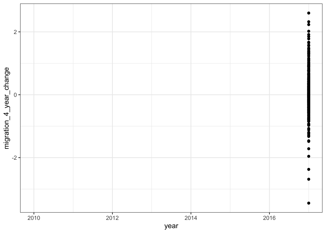
percentage_excessive_drinking and migration_4_year_change only have data from 2017. Following the analysis in the HUD report, we will focus on data from 2017.
\(\rightarrow\) Produce a data frame with data only from 2017. Call it df_2017.
Show Answer
df_2017 <- df_hud %>%
  filter(year == 2017)
\(\rightarrow\) Check for missing values in the 2017 data.
Show Answer
skim_without_charts(df_2017)| Name | df_2017 |
| Number of rows | 374 |
| Number of columns | 43 |
| _______________________ | |
| Column type frequency: | |
| character | 1 |
| numeric | 42 |
| ________________________ | |
| Group variables | None |
Variable type: character
| skim_variable | n_missing | complete_rate | min | max | empty | n_unique | whitespace |
|---|---|---|---|---|---|---|---|
| coc_number | 0 | 1 | 6 | 7 | 0 | 374 | 0 |
Variable type: numeric
| skim_variable | n_missing | complete_rate | mean | sd | p0 | p25 | p50 | p75 | p100 |
|---|---|---|---|---|---|---|---|---|---|
| year | 0 | 1 | 2017.00 | 0.00 | 2017.00 | 2017.00 | 2017.00 | 2017.00 | 2017.00 |
| total_homeless | 0 | 1 | 1466.07 | 5114.12 | 10.00 | 282.75 | 567.50 | 1203.00 | 76501.00 |
| total_sheltered | 0 | 1 | 961.68 | 3921.31 | 5.00 | 189.00 | 373.00 | 850.75 | 72565.00 |
| total_unsheltered | 0 | 1 | 504.39 | 2334.30 | 0.00 | 37.00 | 109.50 | 384.00 | 42828.00 |
| total_population | 0 | 1 | 862794.07 | 1257003.13 | 29344.00 | 271652.75 | 498140.50 | 924319.75 | 11058958.00 |
| house_price_index_2009 | 0 | 1 | 6.90 | 14.68 | -17.53 | -2.61 | 3.12 | 13.51 | 63.86 |
| log_median_rent | 0 | 1 | 2.02 | 0.31 | 1.36 | 1.80 | 1.98 | 2.20 | 2.87 |
| utility_costs | 0 | 1 | 14.84 | 2.97 | 5.90 | 12.95 | 14.97 | 17.16 | 22.60 |
| percentage_owners_cost_burden_2016 | 0 | 1 | 14.88 | 3.04 | 8.07 | 12.49 | 14.40 | 17.09 | 22.96 |
| percentage_renters_severe_cost_burden_2016 | 0 | 1 | 25.55 | 3.87 | 16.38 | 22.89 | 25.00 | 27.82 | 37.65 |
| share_renters_2016 | 0 | 1 | 34.57 | 8.26 | 15.10 | 28.58 | 33.53 | 39.71 | 69.22 |
| rental_vacancy_rate | 0 | 1 | 6.47 | 2.73 | 1.92 | 4.78 | 6.24 | 7.61 | 21.05 |
| high_housing_density | 0 | 1 | 0.25 | 0.44 | 0.00 | 0.00 | 0.00 | 1.00 | 1.00 |
| number_eviction | 0 | 1 | 2402.04 | 4297.43 | 0.00 | 75.75 | 854.50 | 2441.00 | 36357.00 |
| share_overcrowded_units_2016 | 0 | 1 | 2.71 | 1.96 | 0.66 | 1.51 | 2.04 | 3.05 | 12.26 |
| city_or_urban | 0 | 1 | 0.28 | 0.45 | 0.00 | 0.00 | 0.00 | 1.00 | 1.00 |
| suburban | 0 | 1 | 0.43 | 0.50 | 0.00 | 0.00 | 0.00 | 1.00 | 1.00 |
| rate_unemployment | 0 | 1 | 5.00 | 1.57 | 2.51 | 4.14 | 4.90 | 5.57 | 23.64 |
| gini_coefficient_2016 | 0 | 1 | 45.53 | 2.86 | 37.56 | 43.71 | 45.40 | 47.00 | 54.78 |
| poverty_rate | 0 | 1 | 13.41 | 4.14 | 3.50 | 10.50 | 13.23 | 16.08 | 25.56 |
| share_HUD_units | 0 | 1 | 3.53 | 1.84 | 0.09 | 2.24 | 3.22 | 4.57 | 11.86 |
| HUD_unit_occupancy_rate | 0 | 1 | 92.42 | 4.08 | 73.00 | 90.13 | 93.00 | 95.00 | 100.00 |
| share_built_before_1940 | 0 | 1 | 13.04 | 10.52 | 0.26 | 4.58 | 9.91 | 19.21 | 56.01 |
| total_black | 0 | 1 | 107580.71 | 207495.53 | 244.00 | 11811.25 | 37467.50 | 113661.50 | 1909362.00 |
| total_latino_hispanic | 0 | 1 | 154259.52 | 431612.58 | 344.00 | 17374.50 | 39273.00 | 100622.25 | 4924272.00 |
| total_asian | 0 | 1 | 47716.18 | 128225.20 | 106.00 | 5367.00 | 12655.50 | 34762.75 | 1474987.00 |
| total_pacific_islander | 0 | 1 | 1512.28 | 5793.14 | 1.00 | 130.00 | 290.50 | 697.25 | 88323.00 |
| total_population_0_19 | 0 | 1 | 219133.87 | 329833.51 | 6194.00 | 67203.00 | 125673.00 | 236132.50 | 3204024.00 |
| total_population_65_plus | 0 | 1 | 131381.43 | 180215.56 | 6218.00 | 42612.75 | 75493.50 | 138750.00 | 1525916.00 |
| total_female_population | 0 | 1 | 437977.63 | 638095.05 | 14823.00 | 137737.75 | 252411.00 | 473421.25 | 5542088.00 |
| net_migration | 0 | 1 | 3030.79 | 10140.42 | -41321.00 | -990.25 | 442.00 | 3645.50 | 91270.00 |
| migration_4_year_change | 0 | 1 | 0.07 | 0.68 | -3.45 | -0.26 | 0.02 | 0.36 | 2.60 |
| proportion_one_person_households | 0 | 1 | 28.00 | 4.17 | 12.48 | 25.54 | 28.18 | 30.34 | 44.69 |
| share_under_18_with_single_parent | 0 | 1 | 25.76 | 6.89 | 9.77 | 21.02 | 24.81 | 29.44 | 54.47 |
| share_veteran_status | 0 | 1 | 9.94 | 2.86 | 2.80 | 8.16 | 10.07 | 11.28 | 22.27 |
| share_no_bachelors | 0 | 1 | 68.89 | 10.45 | 23.69 | 63.02 | 70.41 | 76.62 | 88.37 |
| medicare_reimbursements_per_enrollee | 0 | 1 | 9.91 | 1.21 | 6.79 | 9.02 | 9.70 | 10.61 | 14.31 |
| percentage_excessive_drinking | 0 | 1 | 0.19 | 0.03 | 0.11 | 0.17 | 0.19 | 0.21 | 0.29 |
| average_Jan_temperature | 0 | 1 | 39.10 | 12.07 | 10.98 | 30.30 | 37.48 | 46.48 | 73.50 |
| average_summer_temperature | 0 | 1 | 75.16 | 5.87 | 59.55 | 71.27 | 75.23 | 79.67 | 93.25 |
| total_Jan_precipitation | 0 | 1 | 4.39 | 3.68 | 0.21 | 2.47 | 3.39 | 4.70 | 25.32 |
| total_annual_precipitation | 0 | 1 | 39.43 | 13.69 | 3.06 | 33.84 | 38.58 | 45.04 | 96.34 |
There are no missing values! We will do our analysis on the 2017 data set.
3.4 Exploratory data analysis
We have two main goals when doing exploratory data analysis. The first is that we want to understand the data set more completely. The second goal is to explore relationships between the variables to help guide the modeling process to answer our specific question.
3.4.1 Graphical summaries
3.4.1.1 Look at the distributions of the homeless counts
\(\rightarrow\) Make a histogram of the total number of homeless in 2017.
Show Answer
df_2017 %>%
  ggplot(aes(x = total_homeless)) +
  geom_histogram(boundary = 0) +
  labs(x = "Total homeless", y = "Count")
## `stat_bin()` using `bins = 30`. Pick better value with `binwidth`.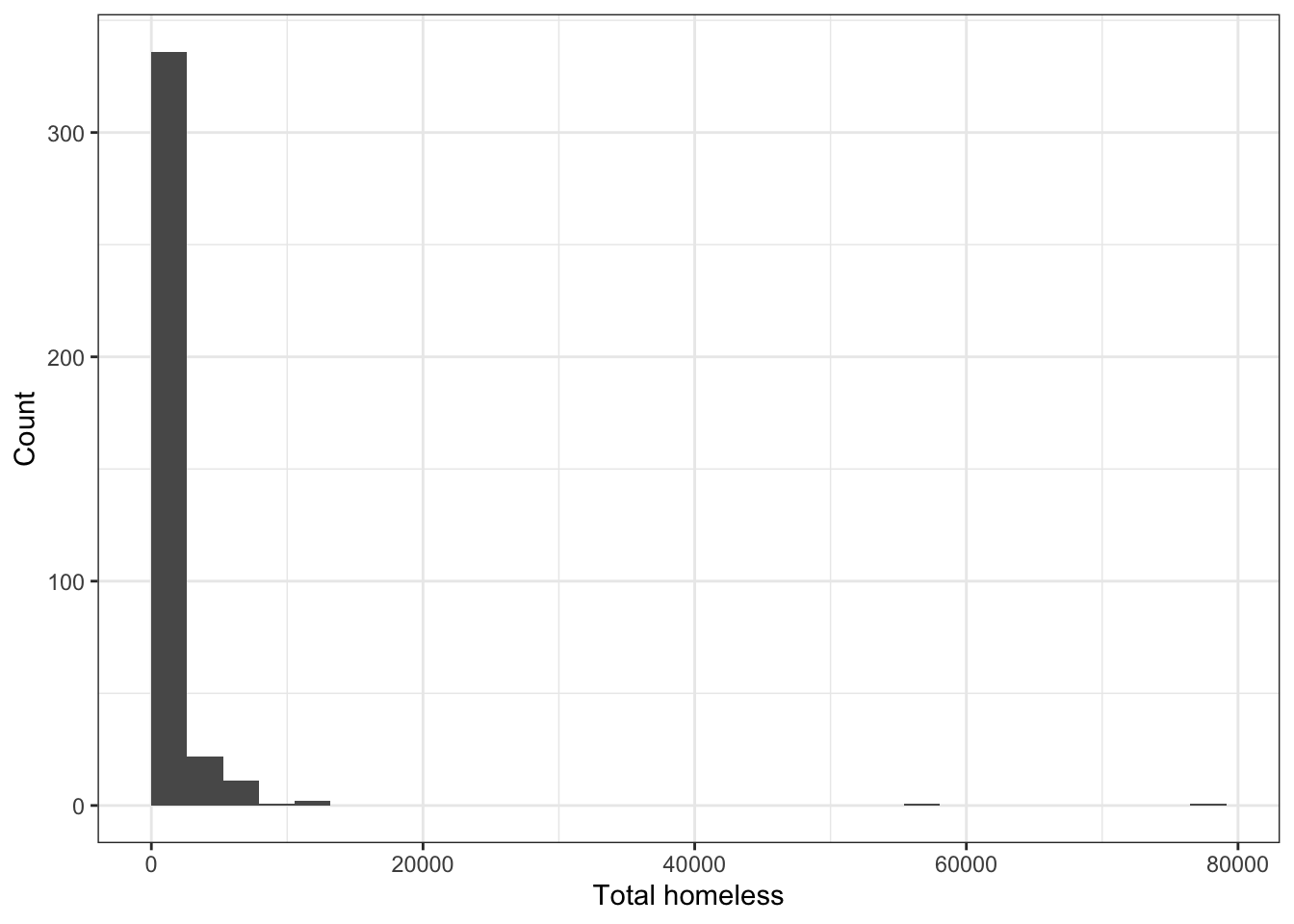 It appears that there are some outliers, but it can be hard to see because of the limits of the y-axis. We can limit the y-axis values to get a better view of the small bars.
df_2017 %>%
  ggplot(aes(x = total_homeless)) +
  geom_histogram(boundary = 0) +
  labs(x = "Total homeless", y = "Count") +
  coord_cartesian(ylim = c(0, 15))
## `stat_bin()` using `bins = 30`. Pick better value with `binwidth`.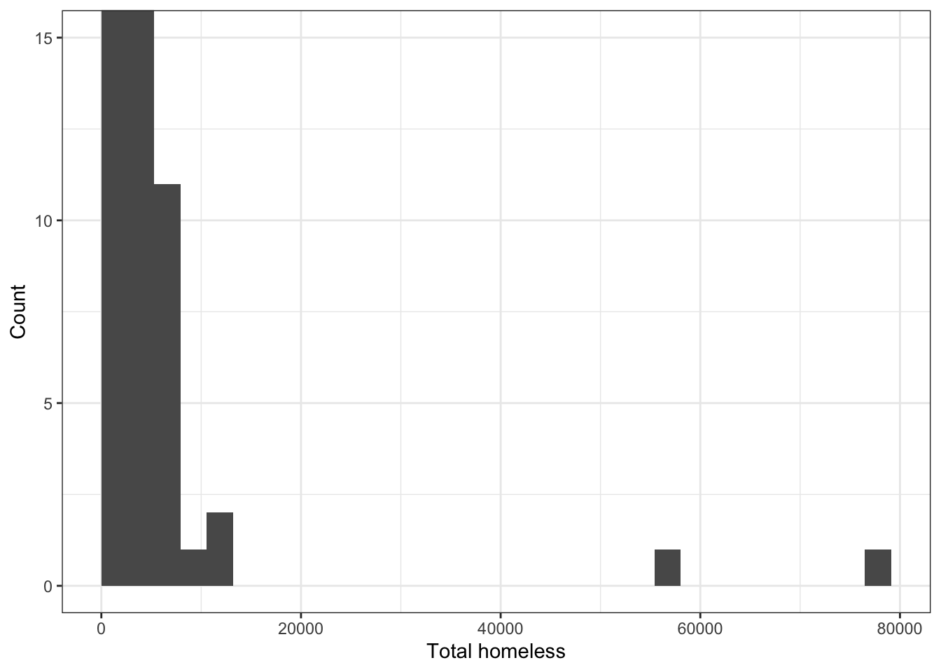
There are some large outliers because there is a wide range of populations among the areas represented in the data set. We can see this by making a histogram of total_population.
df_2017 %>%
  ggplot(aes(x = total_population)) +
  geom_histogram(boundary = 0) +
  labs(x = "Total population", y = "Count")
## `stat_bin()` using `bins = 30`. Pick better value with `binwidth`.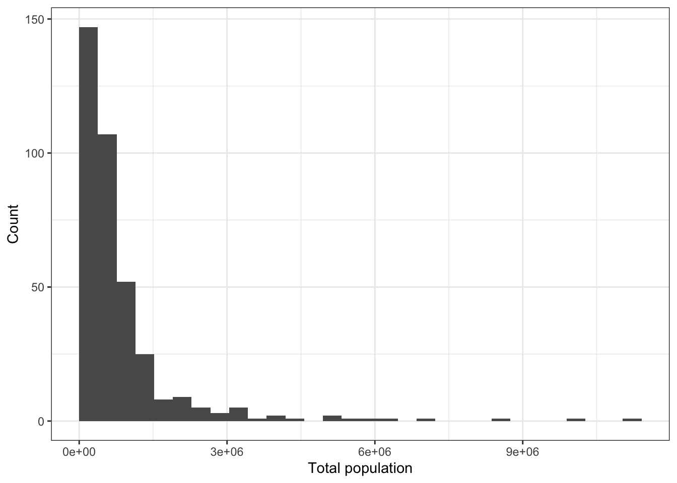
\(\rightarrow\) Make a histogram of the number of sheltered homeless in 2017.
Show Answer
df_2017 %>%
  ggplot(aes(x = total_sheltered)) +
  geom_histogram(boundary = 0) +
  labs(x = "Sheltered homeless", y = "Count")
## `stat_bin()` using `bins = 30`. Pick better value with `binwidth`.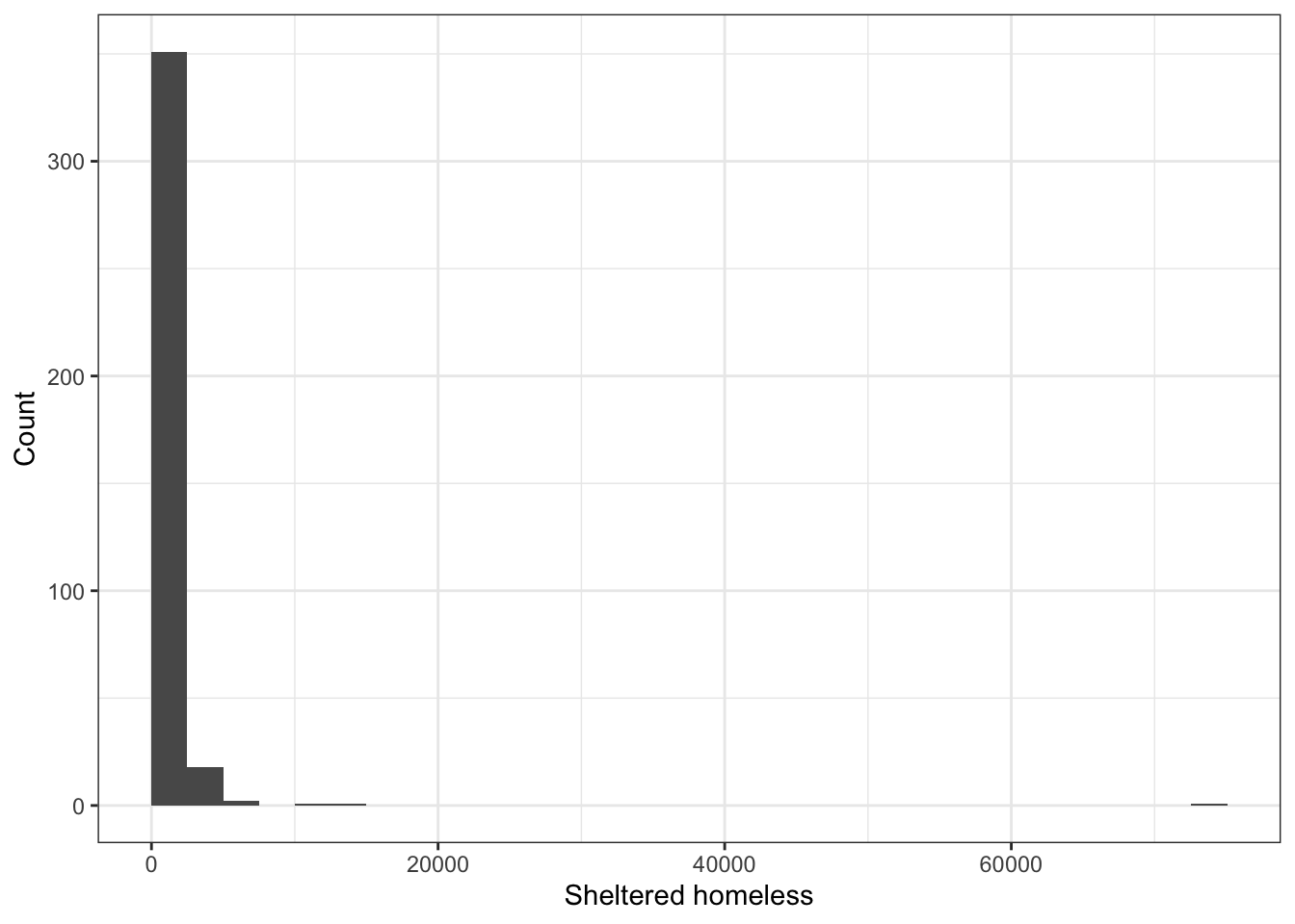
\(\rightarrow\) Make a histogram of the number of unsheltered homeless in 2017.
Show Answer
df_2017 %>%
  ggplot(aes(x = total_unsheltered)) +
  geom_histogram(boundary = 0) +
  labs(x = "Unsheltered homeless", y = "Count")
## `stat_bin()` using `bins = 30`. Pick better value with `binwidth`.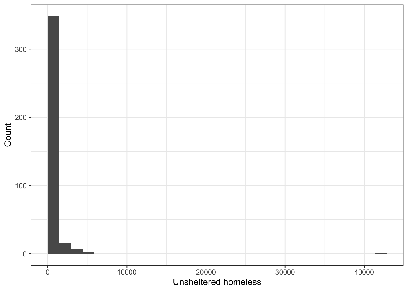
Converting the total counts to rates relative to population size should remove extreme outliers.
\(\rightarrow\) Use the mutate function to create a new variable rate_homeless that is the total number of homeless per 10,000 people in the population and make a histogram of rate_homeless.
Show Answer
df_2017 %>%
  mutate(rate_homeless = total_homeless/(total_population/10000)) %>%
  ggplot(aes(x = rate_homeless)) +
  geom_histogram(boundary = 0) +
  labs(x = "Homeless rate per 10,000", y = "Count")
## `stat_bin()` using `bins = 30`. Pick better value with `binwidth`.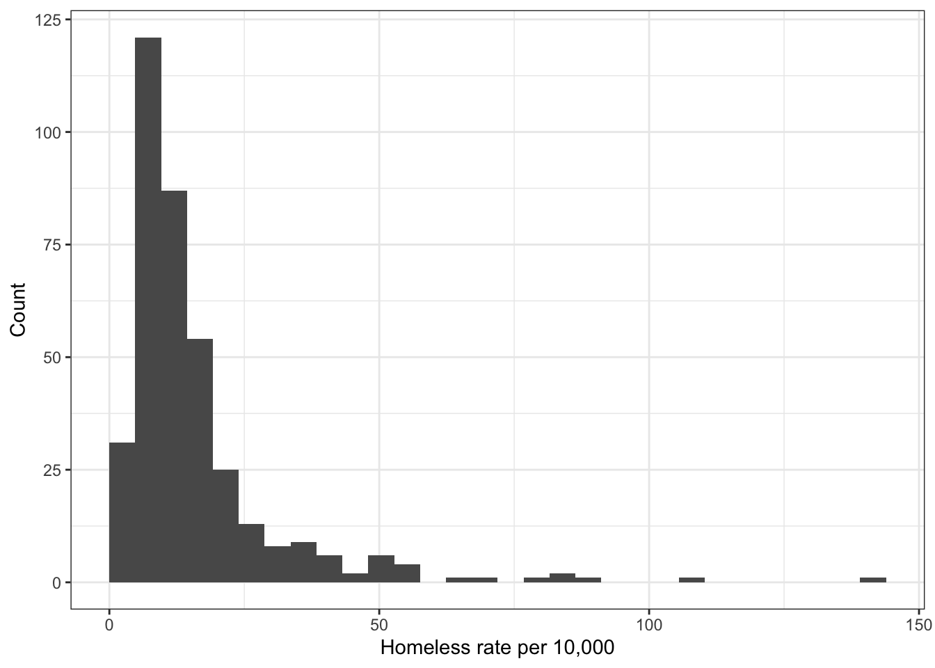
\(\rightarrow\) Compare boxplots of rate_homeless and total_homeless to visually assess whether outliers are less extreme in rate_homeless than in total_homeless.
Show Answer
#Boxplot of rate_homeless
p1 <- df_2017 %>%
  mutate(rate_homeless = total_homeless/(total_population/10000)) %>%
  ggplot() +
  geom_boxplot(aes(y = rate_homeless))

#Boxplot of total_homeless
p2 <- df_2017 %>%
  ggplot() +
  geom_boxplot(aes(y = total_homeless))

#Display as two panels in one graph
grid.arrange(p1, p2, nrow = 1)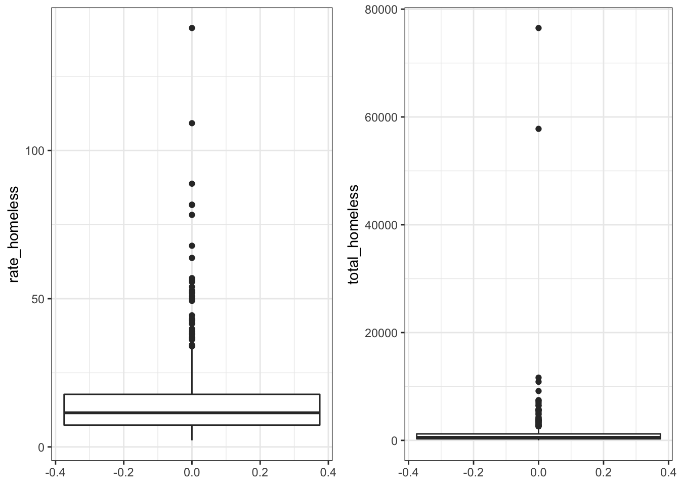
There are still points that are outliers in the rates, but they are not as extreme as in the totals.
3.4.1.2 Data processing
We will add rates to the data frame. Following the HUD report, we will produce rates per 10,000 people.
\(\rightarrow\) Use the mutate function to create new variables rate_homeless, rate_sheltered, and rate_unsheltered in the data frame df_2017 that are the counts per 10,000 people in the population.
Show Answer
df_2017 <- df_2017 %>%
  mutate(rate_sheltered = total_sheltered/(total_population/10000),
         rate_unsheltered = total_unsheltered/(total_population/10000),
         rate_homeless = total_homeless/(total_population/10000))
We should note that the demographic variables (race, gender, age) are given as total counts. We will also convert these totals to percentages.
\(\rightarrow\) Use the mutate function to create new demographics variables in the data frame df_2017 that are percentages of the total population.
Show Answer
df_2017 <- df_2017 %>%
  mutate(percent_black = total_black/total_population,
  percent_latino_hispanic = total_latino_hispanic/total_population,
  percent_asian = total_asian/total_population,
  percent_pacific_islander = total_pacific_islander/total_population,
  percent_population_0_19 = total_population_0_19/total_population,
  percent_population_65_plus = total_population_65_plus/total_population,
  percent_female_population = total_female_population/total_population)
3.4.1.3 Basic summary
\(\rightarrow\) How many people were experiencing homelessness in 2017? How many were sheltered and how many were unsheltered?
Show Answer
df_2017 %>%
  select(total_homeless, total_unsheltered, total_sheltered) %>%
  colSums()
## total_homeless total_unsheltered total_sheltered
## 548312 188643 359669\(\rightarrow\) What are the minimum, maximum, mean, and median number of total, sheltered, and unsheltered homeless in 2017?
Show Answer
df_2017 %>%
  select(total_homeless, total_unsheltered, total_sheltered) %>%
  pivot_longer(cols = c(total_homeless, total_unsheltered, total_sheltered), names_to = "variable", values_to = "count") %>%
  group_by(variable) %>%
  summarize(min = min(count), max = max(count), mean = round(mean(count),1), median = median(count))
## # A tibble: 3 × 5
## variable min max mean median
## <chr> <dbl> <dbl> <dbl> <dbl>
## 1 total_homeless 10 76501 1466. 568.
## 2 total_sheltered 5 72565 962. 373
## 3 total_unsheltered 0 42828 504. 110.3.4.2 Correlations between numerical variables
\(\rightarrow\) Plot the correlation coefficients between all pairs of numerical variables using the corrplot function.
Show Answer
Try this first with no optional arguments in corrplot and notice the problems.
df_2017%>%
  select_if(is.numeric) %>%
  cor(use = "pairwise.complete.obs") %>%
  corrplot()
## Warning in cor(., use = "pairwise.complete.obs"): the standard deviation is zero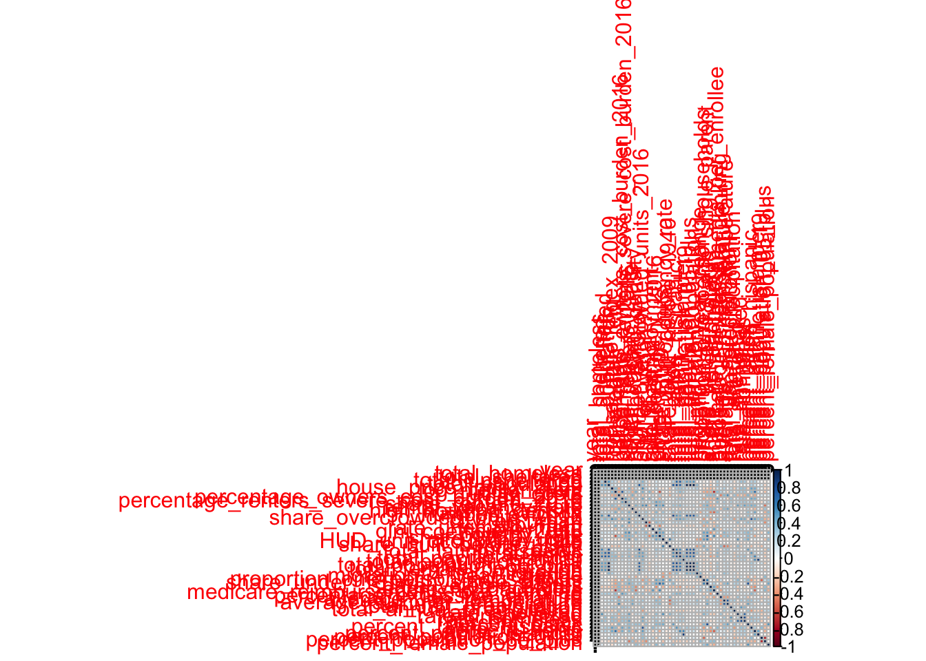
There are two problems. First, year is only equal to 2017, so it doesn’t make sense to compute a correlation coefficient with this variable. So, year should be removed. Also, the labels are huge, so we can’t read the plot.
Try this:
df_2017 %>%
  select_if(is.numeric) %>%
  select(-"year") %>%
  cor(use = "pairwise.complete.obs") %>%
  corrplot(tl.cex = 0.5, type = "lower")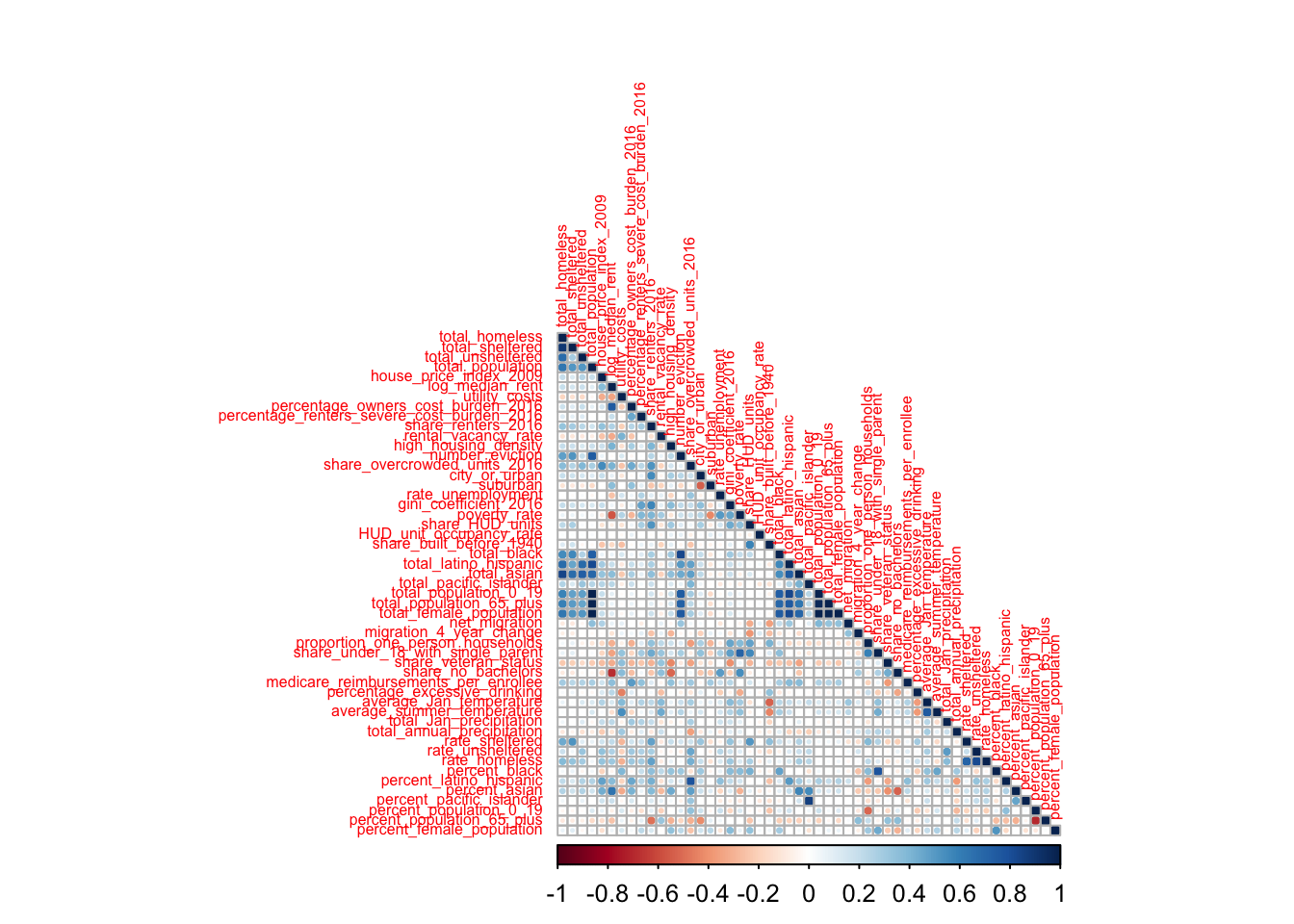
There are some variables that are highly correlated with the rate of homeless. Some are obvious, such as the rate of sheltered homeless. Other correlations show the existence of environmental variables, such as the share of overcrowded units, that are correlated with the rate of homeless.
Note the high correlation among subsets of the input variables. We will want to remove redundant variables or make a transformation of the input variables to deal with the correlation before constructing a model.
Next, we will find the variables with the highest correlation with rate_homeless. First, create the correlation matrix. Then examine the row with rate_homeless to find its correlation with the other variables.
M <- df_2017 %>%
  select_if(is.numeric) %>%
  cor(use = "pairwise.complete.obs")
## Warning in cor(., use = "pairwise.complete.obs"): the standard deviation is zeroround(M["rate_homeless",],2)## year total_homeless
## NA 0.39
## total_sheltered total_unsheltered
## 0.33 0.29
## total_population house_price_index_2009
## 0.05 0.34
## log_median_rent utility_costs
## 0.31 -0.31
## percentage_owners_cost_burden_2016 percentage_renters_severe_cost_burden_2016
## 0.32 0.30
## share_renters_2016 rental_vacancy_rate
## 0.48 -0.08
## high_housing_density number_eviction
## 0.08 0.03
## share_overcrowded_units_2016 city_or_urban
## 0.42 0.19
## suburban rate_unemployment
## -0.12 0.13
## gini_coefficient_2016 poverty_rate
## 0.31 0.13
## share_HUD_units HUD_unit_occupancy_rate
## 0.27 -0.08
## share_built_before_1940 total_black
## 0.09 0.07
## total_latino_hispanic total_asian
## 0.14 0.28
## total_pacific_islander total_population_0_19
## 0.23 0.02
## total_population_65_plus total_female_population
## 0.03 0.05
## net_migration migration_4_year_change
## -0.04 0.03
## proportion_one_person_households share_under_18_with_single_parent
## 0.21 0.11
## share_veteran_status share_no_bachelors
## -0.13 -0.07
## medicare_reimbursements_per_enrollee percentage_excessive_drinking
## 0.11 0.19
## average_Jan_temperature average_summer_temperature
## 0.15 -0.14
## total_Jan_precipitation total_annual_precipitation
## 0.37 -0.03
## rate_sheltered rate_unsheltered
## 0.72 0.83
## rate_homeless percent_black
## 1.00 -0.04
## percent_latino_hispanic percent_asian
## 0.28 0.25
## percent_pacific_islander percent_population_0_19
## 0.22 -0.20
## percent_population_65_plus percent_female_population
## 0.00 -0.08Find the variables where the absolute value of the correlation with rate_homeless is greater than 0.3.
M["rate_homeless",abs(M["rate_homeless",]) > 0.3 & is.na(M["rate_homeless",]) == FALSE] %>%
  abs() %>%
  round(2) %>%
  sort(decreasing = T)
## rate_homeless rate_unsheltered rate_sheltered
## 1.00 0.83 0.72
## share_renters_2016 share_overcrowded_units_2016 total_homeless
## 0.48 0.42 0.39
## total_Jan_precipitation house_price_index_2009 total_sheltered
## 0.37 0.34 0.33
## percentage_owners_cost_burden_2016 log_median_rent utility_costs
## 0.32 0.31 0.31
## gini_coefficient_2016
## 0.31\(\rightarrow\) Make a pairs plot with a subset of the variables with the highest magnitude correlations. Select a small enough group so that you can see the panels. Do not include variables that you will not use as predictors (e.g. rate_unsheltered, any demographic totals)
Show Answer
df_2017 %>%
  select("rate_homeless", "share_renters_2016", "share_overcrowded_units_2016", "total_Jan_precipitation", "house_price_index_2009", "percentage_owners_cost_burden_2016", "log_median_rent", "utility_costs", "gini_coefficient_2016") %>%
  filter("coc_number" != "CA-613") %>%
  ggpairs(progress = FALSE, lower = list(continuous = "cor"), upper = list(continuous = "points"))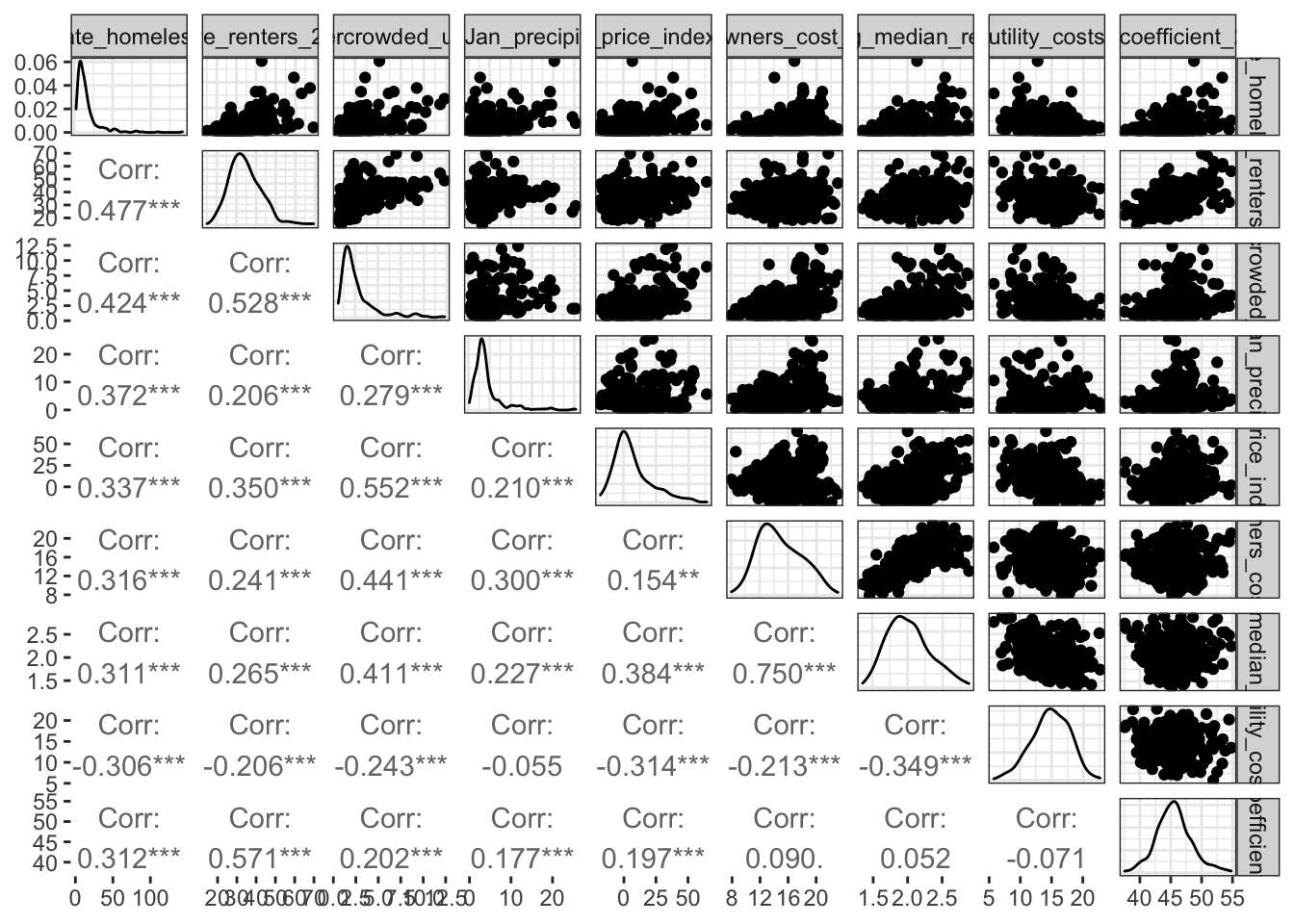
\(\rightarrow\) Create additional plots to further understand the data set. Describe your findings.
3.5 Model
We will multiple approaches to construct models that predict rate_homeless:
- Use statistical significance to create a multiple linear regression model.
- Best subset selection for a multiple linear regression model.
- Lasso
- Ridge regression
- XGBoost
To compare the different approaches, we will use a training and testing split of the data set.
3.5.1 Set up the data set for training and testing
3.5.1.1 Remove some variables
There are several variables that we do not want to include as predictors. We want to remove demographic totals, the year, the CoC number, and the other homeless rates that we are not predicting. You may have additional variables to remove to create the data set that contains only the response variable and the predictors that you want to use.
variable_remove = c("total_homeless", "total_sheltered", "total_unsheltered", "total_black", "total_latino_hispanic", "total_asian", "total_pacific_islander", "total_population_0_19", "total_population_65_plus", "total_female_population", "year", "coc_number", "total_population", "rate_unsheltered", "rate_sheltered")

df_model <- df_2017 %>%
  select(-all_of(variable_remove))

names(df_model)
## [1] "house_price_index_2009" "log_median_rent"
## [3] "utility_costs" "percentage_owners_cost_burden_2016"
## [5] "percentage_renters_severe_cost_burden_2016" "share_renters_2016"
## [7] "rental_vacancy_rate" "high_housing_density"
## [9] "number_eviction" "share_overcrowded_units_2016"
## [11] "city_or_urban" "suburban"
## [13] "rate_unemployment" "gini_coefficient_2016"
## [15] "poverty_rate" "share_HUD_units"
## [17] "HUD_unit_occupancy_rate" "share_built_before_1940"
## [19] "net_migration" "migration_4_year_change"
## [21] "proportion_one_person_households" "share_under_18_with_single_parent"
## [23] "share_veteran_status" "share_no_bachelors"
## [25] "medicare_reimbursements_per_enrollee" "percentage_excessive_drinking"
## [27] "average_Jan_temperature" "average_summer_temperature"
## [29] "total_Jan_precipitation" "total_annual_precipitation"
## [31] "rate_homeless" "percent_black"
## [33] "percent_latino_hispanic" "percent_asian"
## [35] "percent_pacific_islander" "percent_population_0_19"
## [37] "percent_population_65_plus" "percent_female_population"\(\rightarrow\) How many input variables remain in the data set that you can use as predictors?
Show Answer
ncol(df_model) - 1## [1] 37There are 37 input variables.
3.5.1.2 Get train and test splits
We will split the data into training and testing sets, with 85% of the data kept for training.
#Do the split. Keep 85% for training. Use stratified sampling based on rate_homeless
set.seed(20)
split <- initial_split(df_model, prop = 0.85, strata = rate_homeless)

#Extract the training and testing splits
df_train <- training(split)
df_test <- testing(split)
\(\rightarrow\) Check the sizes of the training and testing splits
Show Answer
dim(df_train)## [1] 316 38dim(df_test)## [1] 58 383.5.2 Full regression model
3.5.2.1 Fit the model on the training data
\(\rightarrow\) Use the training data to fit a multiple linear regression model to predict rate_homeless using all possible predictor variables.
Show Coding Hint
Use the lm function:
fit <- lm()Show Answer
fit <- lm(rate_homeless ~ ., df_train)\(\rightarrow\) Examine the summary of the fit. Which predictors have statistically significant coefficients? Do the signs of the coefficients make sense?
Show Answer
summary(fit)##
## Call:
## lm(formula = rate_homeless ~ ., data = df_train)
##
## Residuals:
## Min 1Q Median 3Q Max
## -34.128 -5.250 -0.639 4.658 77.227
##
## Coefficients:
## Estimate Std. Error t value Pr(>|t|)
## (Intercept) -8.630e+01 7.408e+01 -1.165 0.245058
## house_price_index_2009 8.148e-02 6.847e-02 1.190 0.235077
## log_median_rent 3.066e+01 7.959e+00 3.852 0.000146 ***
## utility_costs -1.534e-01 3.674e-01 -0.418 0.676600
## percentage_owners_cost_burden_2016 -1.980e-01 5.030e-01 -0.394 0.694100
## percentage_renters_severe_cost_burden_2016 -7.813e-02 2.803e-01 -0.279 0.780661
## share_renters_2016 1.313e-01 2.302e-01 0.570 0.568882
## rental_vacancy_rate 1.027e-01 3.422e-01 0.300 0.764296
## high_housing_density -3.113e+00 2.257e+00 -1.379 0.168943
## number_eviction 1.765e-04 1.695e-04 1.041 0.298659
## share_overcrowded_units_2016 1.961e+00 8.910e-01 2.201 0.028584 *
## city_or_urban -1.319e+00 2.481e+00 -0.532 0.595463
## suburban -4.344e+00 2.259e+00 -1.923 0.055511 .
## rate_unemployment -7.330e-01 7.791e-01 -0.941 0.347614
## gini_coefficient_2016 1.638e-01 4.853e-01 0.338 0.735922
## poverty_rate -2.161e-01 5.039e-01 -0.429 0.668308
## share_HUD_units 2.040e+00 7.314e-01 2.789 0.005655 **
## HUD_unit_occupancy_rate -9.037e-02 1.700e-01 -0.532 0.595347
## share_built_before_1940 4.870e-02 1.192e-01 0.409 0.683136
## net_migration -1.186e-04 7.745e-05 -1.532 0.126764
## migration_4_year_change 4.159e+00 1.218e+00 3.414 0.000736 ***
## proportion_one_person_households 1.394e+00 4.198e-01 3.319 0.001022 **
## share_under_18_with_single_parent 4.269e-01 3.274e-01 1.304 0.193394
## share_veteran_status 3.439e-02 4.078e-01 0.084 0.932852
## share_no_bachelors 2.719e-01 2.172e-01 1.252 0.211522
## medicare_reimbursements_per_enrollee -5.274e-02 8.654e-01 -0.061 0.951451
## percentage_excessive_drinking 3.351e+01 3.440e+01 0.974 0.330951
## average_Jan_temperature 1.973e-01 1.740e-01 1.134 0.257909
## average_summer_temperature -2.084e-01 3.013e-01 -0.692 0.489812
## total_Jan_precipitation 9.512e-01 2.519e-01 3.777 0.000194 ***
## total_annual_precipitation 7.055e-02 6.875e-02 1.026 0.305695
## percent_black -3.948e+01 1.482e+01 -2.665 0.008158 **
## percent_latino_hispanic -1.515e+01 1.227e+01 -1.235 0.218042
## percent_asian -4.096e+01 2.356e+01 -1.739 0.083220 .
## percent_pacific_islander 2.220e+02 1.278e+02 1.737 0.083571 .
## percent_population_0_19 4.381e+01 6.449e+01 0.679 0.497519
## percent_population_65_plus -2.935e+00 5.118e+01 -0.057 0.954303
## percent_female_population -7.396e+01 1.107e+02 -0.668 0.504533
## ---
## Signif. codes: 0 '***' 0.001 '**' 0.01 '*' 0.05 '.' 0.1 ' ' 1
##
## Residual standard error: 10.93 on 278 degrees of freedom
## Multiple R-squared: 0.5973, Adjusted R-squared: 0.5437
## F-statistic: 11.15 on 37 and 278 DF, p-value: < 2.2e-16Isolate the predictors that have statistically significant coefficients.
#Name the summary
s <- summary(fit)

#Use logical indexing on the matrix of coefficients to find coefficients where the p-value < 0.05
s$coefficients[s$coefficients[,4] < 0.05,1] %>%
  round(2) %>%     #Round because we don't need to look at a million decimal places
  data.frame()     #Create a data frame because it produces a nicer display
## .
## log_median_rent 30.66
## share_overcrowded_units_2016 1.96
## share_HUD_units 2.04
## migration_4_year_change 4.16
## proportion_one_person_households 1.39
## total_Jan_precipitation 0.95
## percent_black -39.48We should also do a qualitative assessment of the fit to the training data.
\(\rightarrow\) Plot the residuals to look for systematic patterns of residuals that might suggest a new model.
Show Answer
plot(fit,1)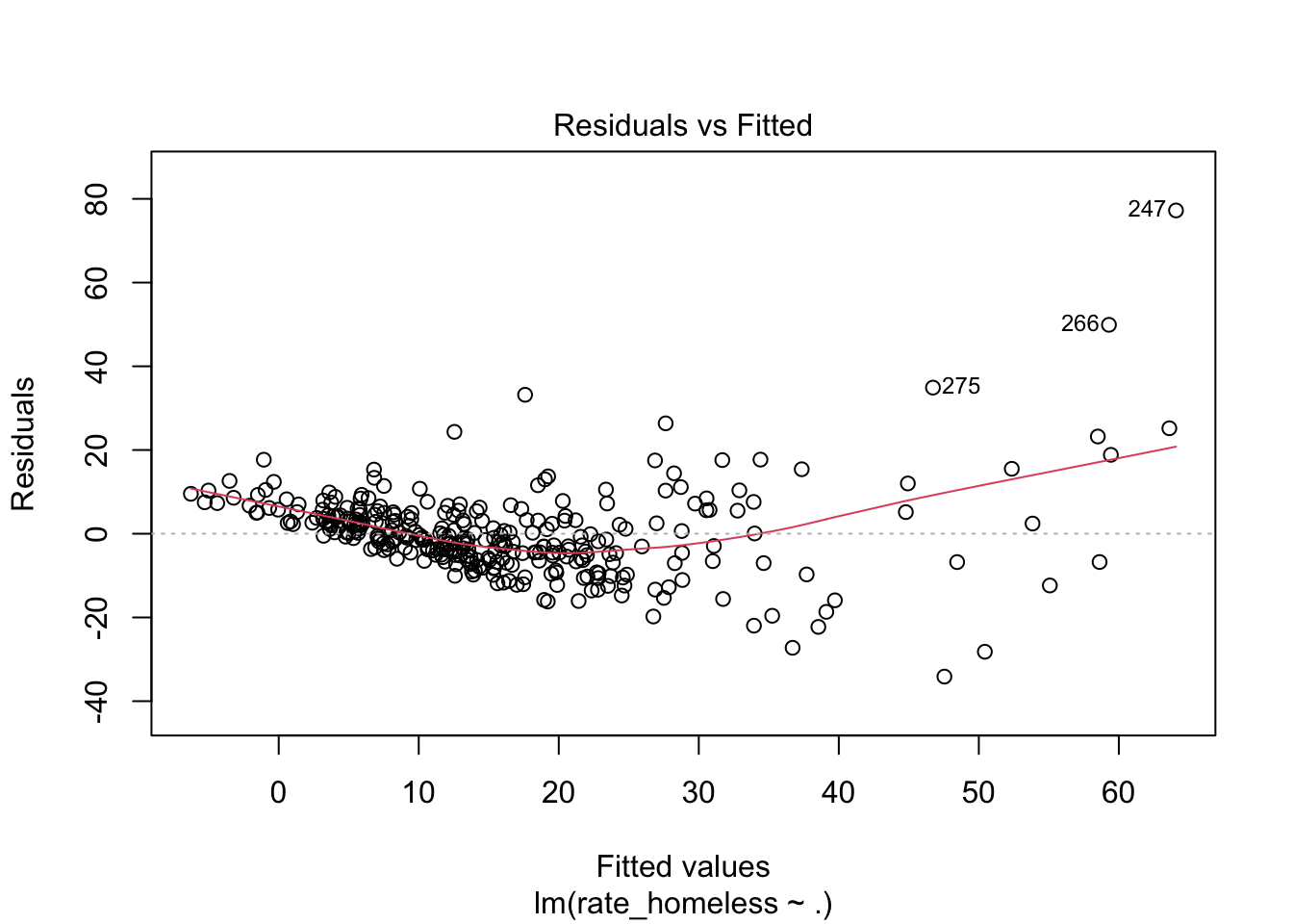
The residual plot has a systematic pattern. How might you use this to alter the model? This is something to explore in the Additional Step.
3.5.2.2 Assess the model on the testing data
\(\rightarrow\) Use the model to predict the homeless rate in the testing data.Coding Hint
Use the function predict to make the predictions.
Show Answer
lm_pred <- predict(fit, df_test)\(\rightarrow\) Make a scatter plot to compare the actual value and the predicted value of rate_homeless.
Show Answer
plot(df_test$rate_homeless, lm_pred, xlab = "Measured homeless rate", ylab = "Predicted homeless rate", pch = 20)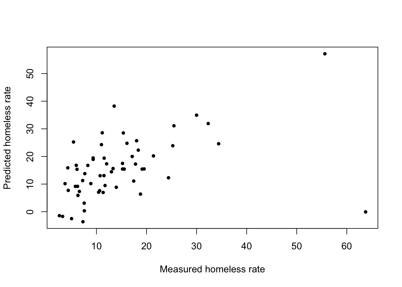
\(\rightarrow\) Compute the RMSE
Show Answer
lm_rmse <- sqrt(mean((df_test$rate_homeless- lm_pred)^2))

lm_rmse
## [1] 11.46046Or, use pipes if you prefer:
lm_rmse <- (df_test$rate_homeless- lm_pred)^2 %>%
  mean() %>%
  sqrt()

lm_rmse
## [1] 11.46046\(\rightarrow\) Repeat the regression analysis, but using a different random seed before the train-test split. Does the train-test split affect the significance of the coefficients and their values?
3.5.3 Subset selection
The full model contains too many predictors, so we will use subset selection on the training data to find a smaller number of predictors.
\(\rightarrow\) Get the number of variables in the data set that will be used as predictors. This will be used to set the subset size.
Show Answer
num_var <- ncol(df_train) - 1\(\rightarrow\) Do best subset selection on the training data. Set the maximum number of variables to equal the number of predictor variables in the data set.
Show Answer
regfit_full <- regsubsets(rate_homeless ~ . , data = df_train, nvmax = num_var)\(\rightarrow\) Get the summary. We will use this after performing cross validation to determine the best model.
Show Answer
reg_summary <- summary(regfit_full)3.5.3.1 Cross validation
\(\rightarrow\) Use 10-fold cross validation on the training data to determine the best subset of predictors in the model.
Show Answer
#Number of observations
n <- nrow(df_train)

#number of folds
k <- 10

#folds
set.seed(1)
#Each observation is randomly assigned to a fold 1, 2, .. k
folds <- sample(1:k,n,replace = TRUE)

#Initialize error for testing data
cv_errors <- matrix(NA,k,num_var,dimnames = list(NULL,paste(1:num_var)))

#For each testing fold
for (j in 1:k){
  #Best subsets on training folds
  reg_fit_best <- regsubsets(rate_homeless ~ ., data = df_train[folds !=j,], nvmax = num_var)

  #test matrix with test fold
  test_mat <- model.matrix(rate_homeless ~ .,data = df_train[folds == j,])

    #Compare errors across models with different numbers of variables
    for (i in 1:num_var){
    #get coefficients of best model with i variables
    coefi <- coef(reg_fit_best,id = i)
    #make predictions using test data
    pred <- test_mat[,names(coefi)] %*% coefi
    #compute test MSE
    cv_errors[j,i] <- mean((df_train$rate_homeless[folds == j] - pred)^2)
  }
}

#Average error over folds
cv_errors_mean <- apply(cv_errors,2,mean)
\(\rightarrow\) Plot the assessment measures vs. the number of predictors
Show Answer
par(mfrow = c(2,2))

ind_cp = which.min(reg_summary$cp)
plot(reg_summary$cp,type = "b",xlab = "Number of variables",ylab = "Cp", main = toString(ind_cp))
points(ind_cp, reg_summary$cp[ind_cp],col = "red",pch = 20)

ind_bic = which.min(reg_summary$bic)
plot(reg_summary$bic,type = "b",xlab = "Number of variables",ylab = "BIC", main = toString(ind_bic))
points(ind_bic, reg_summary$bic[ind_bic],col = "red",pch = 20)

ind_adjr2 = which.max(reg_summary$adjr2)
plot(reg_summary$adjr2,type = "b",xlab = "Number of variables",ylab = "Adjusted R2", main = toString(ind_adjr2))
points(ind_adjr2, reg_summary$adjr2[ind_adjr2],col = "red",pch = 20)

ind_cv <- which.min(cv_errors_mean)
plot(cv_errors_mean,type = "b",xlab = "Number of variables",ylab = "Cross validation", main = toString(ind_cv))
points(ind_cv, cv_errors_mean[ind_cv],col = "red",pch = 20)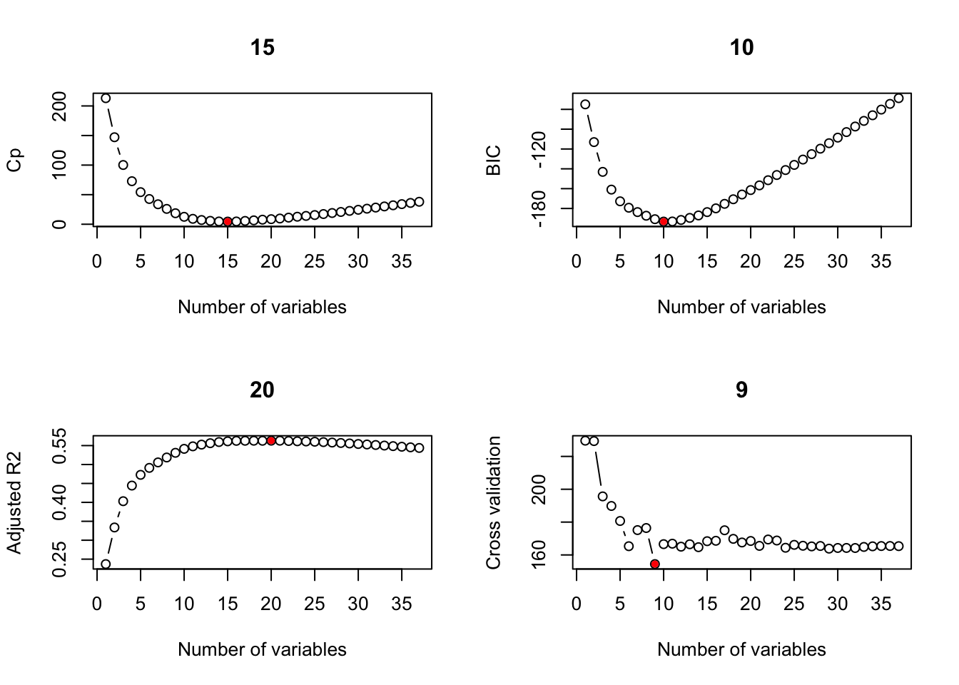
\(\rightarrow\) What are the coefficients of the best model according to different measures?
Show Answer
Try each of: ind_cp, ind_bic, ind_adjr2, ind_cv
coef(regfit_full,ind_cp) %>%
  round(2) %>%
  data.frame()
## .
## (Intercept) -140.81
## log_median_rent 31.22
## percentage_owners_cost_burden_2016 -0.56
## high_housing_density -4.08
## share_overcrowded_units_2016 2.29
## suburban -3.51
## rate_unemployment -1.08
## share_HUD_units 2.36
## migration_4_year_change 3.55
## proportion_one_person_households 1.73
## share_no_bachelors 0.44
## percentage_excessive_drinking 52.57
## total_Jan_precipitation 1.09
## total_annual_precipitation 0.11
## percent_black -21.39
## percent_pacific_islander 211.57coef(regfit_full,ind_bic) %>%
round(2) %>%
data.frame()## .
## (Intercept) -123.86
## log_median_rent 26.78
## share_overcrowded_units_2016 1.49
## suburban -4.31
## share_HUD_units 2.04
## migration_4_year_change 3.79
## proportion_one_person_households 1.80
## share_no_bachelors 0.34
## total_Jan_precipitation 1.12
## percent_black -27.04
## percent_pacific_islander 247.623.5.3.2 Assess the performance of the model on the testing data
Use the model to predict the homeless rate in the testing data. We will use the best BIC model as an example, but you should compare the performance of all models.
\(\rightarrow\) Select the variables that are indicated by the best subset selection criterion that you choose (Cp, BIC, Adjusted R-squared, or CV) and produce a new, smaller data frame.
Show Answer
df_bic <- df_train %>%
  select(all_of(names(coef(regfit_full,ind_bic))[2:length(coef(regfit_full,ind_bic))]), "rate_homeless")

head(df_bic)
## # A tibble: 6 × 11
## log_median_rent share_overcrowded_units_2016 suburban share_HUD_units migration_4_year_ch… proportion_one_…
## <dbl> <dbl> <dbl> <dbl> <dbl> <dbl>
## 1 1.36 1.54 0 4.34 0.232 28.3
## 2 1.44 1.87 0 3.65 0.191 27.3
## 3 1.45 1.98 0 3.75 -0.206 29.2
## 4 1.42 2.49 0 4.71 0.179 30.5
## 5 1.50 2.01 0 2.56 0.630 28.7
## 6 1.89 2.47 0 2.38 0.642 23.6
## # … with 5 more variables: share_no_bachelors <dbl>, total_Jan_precipitation <dbl>, percent_black <dbl>,
## # percent_pacific_islander <dbl>, rate_homeless <dbl>\(\rightarrow\) Fit the model using this subset. The lm object will help us to make predictions easily.
Show Answer
fit_bic <- lm(rate_homeless ~., data = df_bic)

summary(fit_bic)
##
## Call:
## lm(formula = rate_homeless ~ ., data = df_bic)
##
## Residuals:
## Min 1Q Median 3Q Max
## -36.546 -4.824 -1.366 4.441 79.701
##
## Coefficients:
## Estimate Std. Error t value Pr(>|t|)
## (Intercept) -123.8573 15.5886 -7.945 3.77e-14 ***
## log_median_rent 26.7838 3.9648 6.755 7.22e-11 ***
## share_overcrowded_units_2016 1.4937 0.4581 3.261 0.001238 **
## suburban -4.3119 1.4781 -2.917 0.003793 **
## share_HUD_units 2.0380 0.4553 4.477 1.07e-05 ***
## migration_4_year_change 3.7909 1.0552 3.593 0.000381 ***
## proportion_one_person_households 1.8011 0.2065 8.721 < 2e-16 ***
## share_no_bachelors 0.3420 0.1015 3.370 0.000848 ***
## total_Jan_precipitation 1.1238 0.1894 5.934 8.04e-09 ***
## percent_black -27.0435 5.9002 -4.584 6.68e-06 ***
## percent_pacific_islander 247.6198 82.7792 2.991 0.003004 **
## ---
## Signif. codes: 0 '***' 0.001 '**' 0.01 '*' 0.05 '.' 0.1 ' ' 1
##
## Residual standard error: 10.96 on 305 degrees of freedom
## Multiple R-squared: 0.5559, Adjusted R-squared: 0.5414
## F-statistic: 38.18 on 10 and 305 DF, p-value: < 2.2e-16Are all of the coefficients statistically significant?
\(\rightarrow\) Generate predictions of the ACT score in the testing data.
Show Answer
bic_pred <- predict(fit_bic, df_test)\(\rightarrow\) Make a scatter plot to compare the actual value and the predicted value of rate_homeless.
Show Answer
plot(df_test$rate_homeless, bic_pred, xlab = "Measured homeless rate", ylab = "Predicted homeless rate", pch = 20)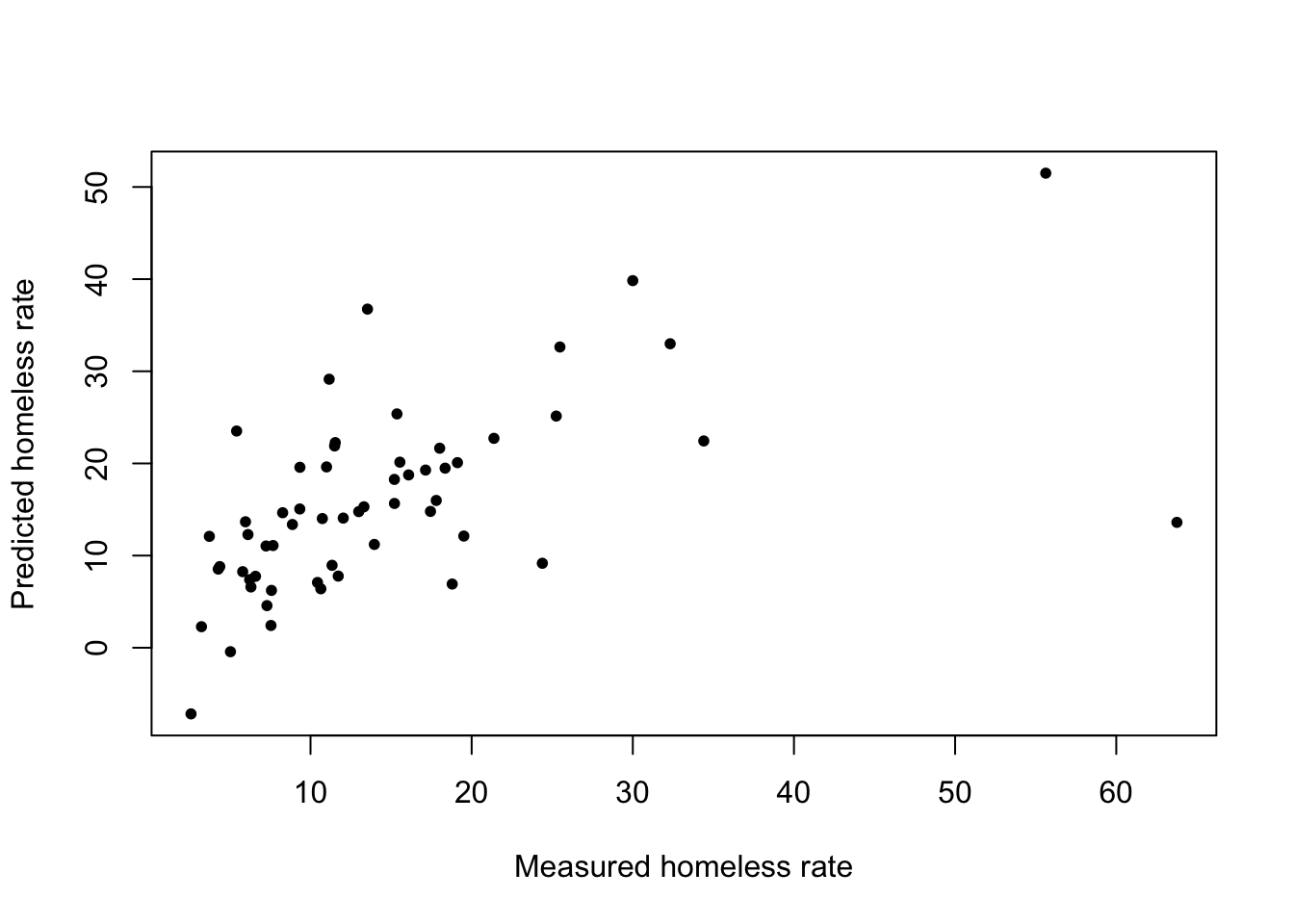
\(\rightarrow\) Compute the RMSE. How does the RMSE compare to the error for the full model?
Show Answer
bic_rmse <- sqrt(mean((df_test$rate_homeless- bic_pred)^2))

bic_rmse
## [1] 9.8173783.5.4 Lasso
The lasso is another approach to producing a linear regression model with a subset of the available predictors. The lasso works by finding coefficients \(\boldsymbol{\beta}\) that minimize the cost function:
\[C(\boldsymbol{\beta}) = \sum_{i=1}^n(y_i - \beta_{0} - \sum_{j=1}^p\beta_{j}x_{ij})^2 + \lambda \sum_{j=1}^p|\beta_{j}| = \text{RSS} + \lambda \sum_{j=1}^p|\beta_{j}|\]
where \(\lambda \geq 0\) is a tuning parameter (or hyperparameter).
\(\rightarrow\) Prepare the data by creating a model matrix x_train from the training data. Create the model matrix using model.matrix so that it includes the training data for all predictors, but does not include a column for the intercept. Also create the training response data y_train.
Show Answer
x_train <- model.matrix(rate_homeless ~ ., df_train)[,-1] #Remove the intercept
y_train <- df_train$rate_homeless
\(\rightarrow\) Use cross-validation to find the best hyperparameter \(\lambda\)
Show Answer
#alpha = 1 says that we will use the lasso
cv_lasso <- cv.glmnet(x_train, y_train, alpha = 1)
\(\rightarrow\) Show error as a function of the hyperparameter \(\lambda\) and its best value.
Show Answer
plot(cv_lasso)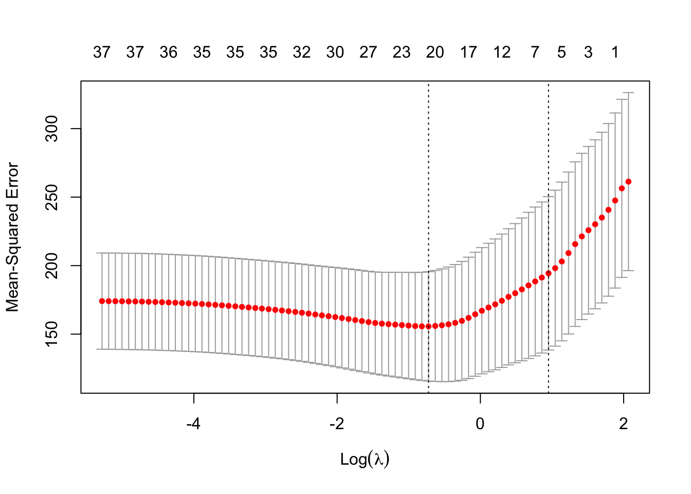
best_lam <- cv_lasso$lambda.min
best_lam
## [1] 0.4849755\(\rightarrow\) Fit the lasso with the best \(\lambda\) using the function glmnet.
Show Answer
lasso_mod <- glmnet(x_train, y_train, alpha = 1, lambda = best_lam)\(\rightarrow\) Examine the coefficients. Which variables have non-zero coefficients?
Show Answer
round(coef(lasso_mod),3)## 38 x 1 sparse Matrix of class "dgCMatrix"
## s0
## (Intercept) -41.161
## house_price_index_2009 0.057
## log_median_rent 13.326
## utility_costs -0.061
## percentage_owners_cost_burden_2016 .
## percentage_renters_severe_cost_burden_2016 .
## share_renters_2016 0.106
## rental_vacancy_rate .
## high_housing_density -2.443
## number_eviction .
## share_overcrowded_units_2016 1.929
## city_or_urban .
## suburban -1.970
## rate_unemployment .
## gini_coefficient_2016 .
## poverty_rate .
## share_HUD_units 1.652
## HUD_unit_occupancy_rate .
## share_built_before_1940 .
## net_migration .
## migration_4_year_change 2.854
## proportion_one_person_households 1.147
## share_under_18_with_single_parent .
## share_veteran_status 0.102
## share_no_bachelors 0.065
## medicare_reimbursements_per_enrollee .
## percentage_excessive_drinking 40.582
## average_Jan_temperature .
## average_summer_temperature -0.005
## total_Jan_precipitation 1.024
## total_annual_precipitation 0.027
## percent_black -9.311
## percent_latino_hispanic .
## percent_asian .
## percent_pacific_islander 208.525
## percent_population_0_19 -40.775
## percent_population_65_plus .
## percent_female_population -43.8913.5.4.1 Look at prediction error
\(\rightarrow\) Use the model to predict the homeless rate in the testing data.
Show Answer
First create a model matrix with the testing data
x_test <- model.matrix(rate_homeless ~ .,df_test)[,-1] #Remove the interceptUse the predict function to make the prediction of the testing ACT data.
lasso_pred <- predict(lasso_mod, s = best_lam, newx = x_test)\(\rightarrow\) Make a scatter plot to compare the actual value and the predicted value of rate_homeless.
Show Answer
plot(df_test$rate_homeless, lasso_pred, xlab = "Measured homeless rate", ylab = "Predicted homeless rate", pch = 20)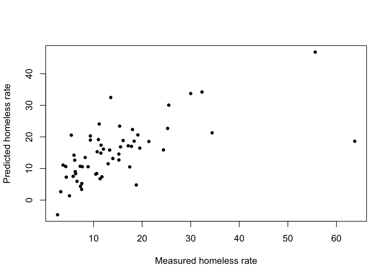
\(\rightarrow\) Compute the RMSE. How does it compare to the other models?
Show Answer
lasso_rmse <- sqrt(mean((df_test$rate_homeless - lasso_pred)^2))
lasso_rmse
## [1] 8.632383.5.5 Ridge regression
Ridge regression is another approach to model building
Ridge regression works by finding coefficients \(\boldsymbol{\beta}\) that minimize the cost function:
\[C(\boldsymbol{\beta}) = \sum_{i=1}^n(y_i - \beta_{0} - \sum_{j=1}^p\beta_{j}x_{ij})^2 + \lambda \sum_{j=1}^p\beta_{j}^2 = \text{RSS} + \lambda \sum_{j=1}^p\beta_{j}^2\]
In contrast to the lasso, ridge regression will not reduce the number of non-zero coefficients in the model. Ridge regression will shrink the coefficients, which helps to prevent overfitting of the training data.
The fitting procedure for the ridge regression model mirrors the lasso approach, only changing the parameter \(\alpha\) to 0 in the cv.glmnet and glmnet functions.
\(\rightarrow\) Fit and assess a ridge regression model. How does it compare to the other models?
Show Answer
First, do cross validation to find the best value of the \(\lambda\)
cv_ridge <- cv.glmnet(x_train,y_train,alpha = 0)

best_lam <- cv_ridge$lambda.min
Fit the model with the best value of the \(\lambda\)
ridge_mod <- glmnet(x_train, y_train, alpha = 0, lambda = best_lam)Predict the ACT scores in the test data
ridge_pred <- predict(ridge_mod, s = best_lam, newx = x_test)Compute the RMSE
ridge_rmse <- sqrt(mean((df_test$rate_homeless - ridge_pred)^2))
ridge_rmse
## [1] 9.472633.5.6 XGBoost
XGBoost is short for eXtreme Gradient Boosting.
We are going to use the tidymodels package to fit the XGBoost model.
3.5.6.1 Set up the model
The model will be a boosted tree model, so we start by specifying the features of a boost_tree model. Theboost_tree creates a specification of a model, but does not fit the model.
xgb_spec <- boost_tree(
  mode = "regression",  #We are solving a regression problem
  trees = 1000,
  tree_depth = tune(),  # tune() says that we will specify this parameter later
  min_n = tune(),
  loss_reduction = tune(),
  sample_size = tune(),
  mtry = tune(),
  learn_rate = tune(),
  ) %>%
  set_engine("xgboost", objective = "reg:squarederror") ## We will use xgboost to fit the model and try to minimize the squared error

xgb_spec
## Boosted Tree Model Specification (regression)
##
## Main Arguments:
## mtry = tune()
## trees = 1000
## min_n = tune()
## tree_depth = tune()
## learn_rate = tune()
## loss_reduction = tune()
## sample_size = tune()
##
## Engine-Specific Arguments:
## objective = reg:squarederror
##
## Computational engine: xgboostCreate a workflow that specifies the model formula and the model type. We are still setting up the model; this does not fit the model.
xgb_wf <- workflow() %>%
add_formula(rate_homeless ~ .) %>%
add_model(xgb_spec)
xgb_wf## ══ Workflow ═════════════════════════════════════════════════════════════════════════════════════════════════
## Preprocessor: Formula
## Model: boost_tree()
##
## ── Preprocessor ─────────────────────────────────────────────────────────────────────────────────────────────
## rate_homeless ~ .
##
## ── Model ────────────────────────────────────────────────────────────────────────────────────────────────────
## Boosted Tree Model Specification (regression)
##
## Main Arguments:
##   mtry = tune()
##   trees = 1000
##   min_n = tune()
##   tree_depth = tune()
##   learn_rate = tune()
##   loss_reduction = tune()
##   sample_size = tune()
##
## Engine-Specific Arguments:
##   objective = reg:squarederror
##
## Computational engine: xgboost3.5.6.2 Fit the model
We need to fit all of the parameters that we specified as tune(). We will specify the parameter grid using the functions grid_latin_hypercube:
xgb_grid <- grid_latin_hypercube(
  tree_depth(),
  min_n(),
  loss_reduction(),
  sample_size = sample_prop(),
  finalize(mtry(), df_train),
  learn_rate(),
  size = 30  #Create 30 sets of the 6 parameters
)
Create folds for cross-validation.
#folds <- vfold_cv(df_train, strata = rate_homeless)

folds <- vfold_cv(df_train)
Do the parameter fitting. This will take some time.
xgb_res <- tune_grid(
  xgb_wf,              #The workflow
  resamples = folds,   #The training data split into folds
  grid = xgb_grid,     #The grid of parameters to fit
  control = control_grid(save_pred = TRUE)
)
## ! Fold01: internal: A correlation computation is required, but `estimate` is constant and has 0 standard deviat...## ! Fold02: internal: A correlation computation is required, but `estimate` is constant and has 0 standard deviat...## ! Fold03: internal: A correlation computation is required, but `estimate` is constant and has 0 standard deviat...## ! Fold04: internal: A correlation computation is required, but `estimate` is constant and has 0 standard deviat...## ! Fold05: internal: A correlation computation is required, but `estimate` is constant and has 0 standard deviat...## ! Fold06: internal: A correlation computation is required, but `estimate` is constant and has 0 standard deviat...## ! Fold07: internal: A correlation computation is required, but `estimate` is constant and has 0 standard deviat...## ! Fold08: internal: A correlation computation is required, but `estimate` is constant and has 0 standard deviat...## ! Fold09: internal: A correlation computation is required, but `estimate` is constant and has 0 standard deviat...## ! Fold10: internal: A correlation computation is required, but `estimate` is constant and has 0 standard deviat...xgb_res## Warning: This tuning result has notes. Example notes on model fitting include:
## internal: A correlation computation is required, but `estimate` is constant and has 0 standard deviation, resulting in a divide by 0 error. `NA` will be returned.
## internal: A correlation computation is required, but `estimate` is constant and has 0 standard deviation, resulting in a divide by 0 error. `NA` will be returned.
## internal: A correlation computation is required, but `estimate` is constant and has 0 standard deviation, resulting in a divide by 0 error. `NA` will be returned.## # Tuning results
## # 10-fold cross-validation
## # A tibble: 10 × 5
## splits id .metrics .notes .predictions
## <list> <chr> <list> <list> <list>
## 1 <split [284/32]> Fold01 <tibble [60 × 10]> <tibble [1 × 1]> <tibble [960 × 10]>
## 2 <split [284/32]> Fold02 <tibble [60 × 10]> <tibble [1 × 1]> <tibble [960 × 10]>
## 3 <split [284/32]> Fold03 <tibble [60 × 10]> <tibble [1 × 1]> <tibble [960 × 10]>
## 4 <split [284/32]> Fold04 <tibble [60 × 10]> <tibble [1 × 1]> <tibble [960 × 10]>
## 5 <split [284/32]> Fold05 <tibble [60 × 10]> <tibble [1 × 1]> <tibble [960 × 10]>
## 6 <split [284/32]> Fold06 <tibble [60 × 10]> <tibble [1 × 1]> <tibble [960 × 10]>
## 7 <split [285/31]> Fold07 <tibble [60 × 10]> <tibble [1 × 1]> <tibble [930 × 10]>
## 8 <split [285/31]> Fold08 <tibble [60 × 10]> <tibble [1 × 1]> <tibble [930 × 10]>
## 9 <split [285/31]> Fold09 <tibble [60 × 10]> <tibble [1 × 1]> <tibble [930 × 10]>
## 10 <split [285/31]> Fold10 <tibble [60 × 10]> <tibble [1 × 1]> <tibble [930 × 10]>Set up the final workflow with the best model parameters.
#Get the best model, according to RMSE
best_rmse <- select_best(xgb_res, "rmse")

#Update the workflow with the best parameters
final_xgb <- finalize_workflow(
  xgb_wf,
  best_rmse
)

final_xgb
## ══ Workflow ═════════════════════════════════════════════════════════════════════════════════════════════════
## Preprocessor: Formula
## Model: boost_tree()
##
## ── Preprocessor ─────────────────────────────────────────────────────────────────────────────────────────────
## rate_homeless ~ .
##
## ── Model ────────────────────────────────────────────────────────────────────────────────────────────────────
## Boosted Tree Model Specification (regression)
##
## Main Arguments:
## mtry = 7
## trees = 1000
## min_n = 3
## tree_depth = 4
## learn_rate = 0.0107153006007263
## loss_reduction = 0.00168670164001662
## sample_size = 0.60449863047339
##
## Engine-Specific Arguments:
## objective = reg:squarederror
##
## Computational engine: xgboost3.5.6.3 Prediction
Fit the final model to the training data.
xgb_fit <- final_xgb %>%
  fit(df_train)
Generate predictions and bind them together with the true values from the test data.
predictions_xgb <- xgb_fit %>%
  predict(new_data = df_test) %>%
  bind_cols(df_test %>% select(rate_homeless))
Show the RMSE. Compare the result to the test RMSE for the other models.
predictions_xgb %>%
  metrics(rate_homeless, .pred)
## # A tibble: 3 × 3
## .metric .estimator .estimate
## <chr> <chr> <dbl>
## 1 rmse standard 9.11
## 2 rsq standard 0.417
## 3 mae standard 5.77Plot the ACT scores and the prediction
plot(df_test$rate_homeless, predictions_xgb$.pred, pch = 20, xlab = "Homeless rate", ylab = "Predicted homeless rate")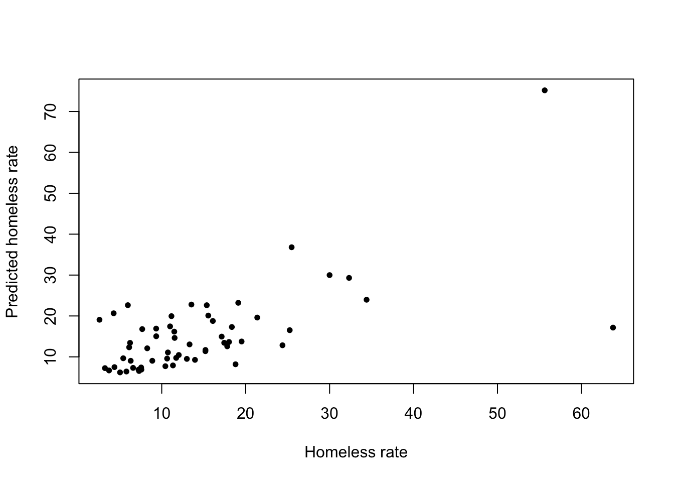
3.5.6.4 Relative importance of predictors
Look at which predictors are most important in the model
xgb_fit %>%
  pull_workflow_fit() %>%
  vip(geom = "col")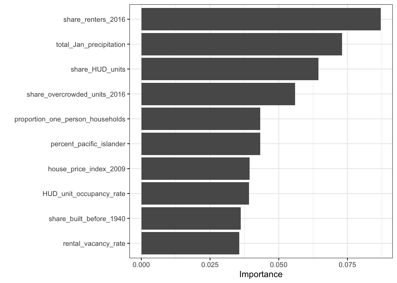
3.5.7 Compare models
You used several methods to construct a model
- Use statistical significance to create a multiple linear regression model.
- Best subset selection for a multiple linear regression model.
- Lasso
- Ridge regression
- XGBoost
Compare the performance of the models.
3.6 Additional step
In addition to completing the above analyses, you should perform any revisions to the models that you think might improve their performance. Consult Canvas for further directions.
3.7 Conclusion
After completing your analyses, you will make your conclusions and communicate your results. Consult Canvas for further directions.