Chapter 2 Education inequality
2.1 Introduction
This project addresses inequality of educational opportunity in U.S. high schools. Here we will focus on average student performance on the ACT or SAT exams that students take as part of the college application process.
We expect a range of school performance on these exams, but is school performance predicted by socioeconomic factors?
2.2 Data Collection
This project utilizes two data sets. The primary data set is the EdGap data set from EdGap.org. This data set from 2016 includes information about average ACT or SAT scores for schools and several socioeconomic characteristics of the school district. The secondary data set is basic information about each school from the National Center for Education Statistics.
2.2.1 EdGap data
All socioeconomic data (household income, unemployment, adult educational attainment, and family structure) are from the Census Bureau’s American Community Survey.
EdGap.org report that ACT and SAT score data is from each state’s department of education or some other public data release. The nature of the other public data release is not known.
The quality of the census data and the department of education data can be assumed to be reasonably high.
EdGap.org do not indicate that they processed the data in any way. The data were assembled by the EdGap.org team, so there is always the possibility for human error. Given the public nature of the data, we would be able to consult the original data sources to check the quality of the data if we had any questions.
2.2.2 School information data
The school information data is from the National Center for Education Statistics. This data set consists of basic identifying information about schools and can be assumed to be of reasonably high quality. As for the EdGap.org data, the school information data is public, so we would be able to consult the original data sources to check the quality of the data if we had any questions.
2.2.3 Data ethics
2.2.3.1 Data Science Ethics Checklist
![]()
A. Problem Formulation
- A.1 Well-Posed Problem: Is it possible to answer our question with data? Is the problem well-posed?
B. Data Collection
- B.1 Informed consent: If there are human subjects, have they given informed consent, where subjects affirmatively opt-in and have a clear understanding of the data uses to which they consent?
- B.2 Collection bias: Have we considered sources of bias that could be introduced during data collection and survey design and taken steps to mitigate those?
- B.3 Limit PII exposure: Have we considered ways to minimize exposure of personally identifiable information (PII) for example through anonymization or not collecting information that isn’t relevant for analysis?
- B.4 Downstream bias mitigation: Have we considered ways to enable testing downstream results for biased outcomes (e.g., collecting data on protected group status like race or gender)?
C. Data Storage
- C.1 Data security: Do we have a plan to protect and secure data (e.g., encryption at rest and in transit, access controls on internal users and third parties, access logs, and up-to-date software)?
- C.2 Right to be forgotten: Do we have a mechanism through which an individual can request their personal information be removed?
- C.3 Data retention plan: Is there a schedule or plan to delete the data after it is no longer needed?
D. Analysis
- D.1 Missing perspectives: Have we sought to address blindspots in the analysis through engagement with relevant stakeholders (e.g., checking assumptions and discussing implications with affected communities and subject matter experts)?
- D.2 Dataset bias: Have we examined the data for possible sources of bias and taken steps to mitigate or address these biases (e.g., stereotype perpetuation, confirmation bias, imbalanced classes, or omitted confounding variables)?
- D.3 Honest representation: Are our visualizations, summary statistics, and reports designed to honestly represent the underlying data?
- D.4 Privacy in analysis: Have we ensured that data with PII are not used or displayed unless necessary for the analysis?
- D.5 Auditability: Is the process of generating the analysis well documented and reproducible if we discover issues in the future?
E. Modeling
- E.1 Proxy discrimination: Have we ensured that the model does not rely on variables or proxies for variables that are unfairly discriminatory?
- E.2 Fairness across groups: Have we tested model results for fairness with respect to different affected groups (e.g., tested for disparate error rates)?
- E.3 Metric selection: Have we considered the effects of optimizing for our defined metrics and considered additional metrics?
- E.4 Explainability: Can we explain in understandable terms a decision the model made in cases where a justification is needed?
- E.5 Communicate bias: Have we communicated the shortcomings, limitations, and biases of the model to relevant stakeholders in ways that can be generally understood?
F. Deployment
- F.1 Redress: Have we discussed with our organization a plan for response if users are harmed by the results (e.g., how does the data science team evaluate these cases and update analysis and models to prevent future harm)?
- F.2 Roll back: Is there a way to turn off or roll back the model in production if necessary?
- F.3 Concept drift: Do we test and monitor for concept drift to ensure the model remains fair over time?
- F.4 Unintended use: Have we taken steps to identify and prevent unintended uses and abuse of the model and do we have a plan to monitor these once the model is deployed?
Data Science Ethics Checklist generated with deon.
We will discuss these issues in class.
2.3 Data Preparation
2.3.1 Load necessary packages
#readxl lets us read Excel files
library(readxl)
#GGally has a nice pairs plotting function
library(GGally)
#skimr provides a nice summary of a data set
library(skimr)
#leaps will be used for model selection
library(leaps)
#kableExtra will be used to make tables in the html document
library(kableExtra)
#latex2exp lets us use LaTex in ggplot
library(latex2exp)
#tidyverse contains packages we will use for processing and plotting data
library(tidyverse)
2.3.2 Load the data
2.3.2.1 Load the EdGap set
\(\rightarrow\) Load the data set contained in the file EdGap_data.xlsx and name the data frame edgap.
Show Coding Hint
Use the function read_excel from the package readxl to load the data.
Show Answer
edgap <- read_excel("EdGap_data.xlsx")2.3.3 Explore the contents of the data set
\(\rightarrow\) Look at the first few rows of the data frame.
Show Coding Hint
You can use the function head to see the head of the data frame.
Show Answer
head(edgap, n = 5)## # A tibble: 5 × 7
## `NCESSCH School ID` `CT Unemployment …` `CT Pct Adults…` `CT Pct Childr…` `CT Median Hou…` `School ACT av…`
## <dbl> <dbl> <dbl> <dbl> <dbl> <dbl>
## 1 100001600143 0.118 0.445 0.346 42820 20.4
## 2 100008000024 0.0640 0.663 0.768 89320 19.5
## 3 100008000225 0.0565 0.702 0.713 84140 19.6
## 4 100017000029 0.0447 0.692 0.641 56500 17.7
## 5 100018000040 0.0770 0.640 0.834 54015 18.2
## # … with 1 more variable: `School Pct Free and Reduced Lunch` <dbl>n = 5 to show the first 5 rows.
Use the View function to explore the full data set.
View(edgap)2.3.3.1 Load school information data
\(\rightarrow\) Load the data set contained in the file ccd_sch_029_1617_w_1a_11212017.csv and name the data frame school_info.
Show Answer
school_info <- read_csv("ccd_sch_029_1617_w_1a_11212017.csv")## Warning: One or more parsing issues, see `problems()` for details## Rows: 102181 Columns: 65
## ── Column specification ─────────────────────────────────────────────────────────────────────────────────────
## Delimiter: ","
## chr (60): SCHOOL_YEAR, FIPST, STATENAME, ST, SCH_NAME, LEA_NAME, STATE_AGENCY_NO, UNION, ST_LEAID, LEAID,...
## dbl (3): SY_STATUS, UPDATED_STATUS, SCH_TYPE
## lgl (2): MSTREET3, LSTREET3
##
## ℹ Use `spec()` to retrieve the full column specification for this data.
## ℹ Specify the column types or set `show_col_types = FALSE` to quiet this message.\(\rightarrow\) Look at the first few rows of the data frame.
Show Answer
head(school_info)## # A tibble: 6 × 65
## SCHOOL_YEAR FIPST STATENAME ST SCH_NAME LEA_NAME STATE_AGENCY_NO UNION ST_LEAID LEAID ST_SCHID NCESSCH
## <chr> <chr> <chr> <chr> <chr> <chr> <chr> <chr> <chr> <chr> <chr> <chr>
## 1 2016-2017 01 ALABAMA AL Sequoyah … Alabama… 01 <NA> AL-210 0100… AL-210-… 010000…
## 2 2016-2017 01 ALABAMA AL Camps Alabama… 01 <NA> AL-210 0100… AL-210-… 010000…
## 3 2016-2017 01 ALABAMA AL Det Ctr Alabama… 01 <NA> AL-210 0100… AL-210-… 010000…
## 4 2016-2017 01 ALABAMA AL Wallace S… Alabama… 01 <NA> AL-210 0100… AL-210-… 010000…
## 5 2016-2017 01 ALABAMA AL McNeel Sc… Alabama… 01 <NA> AL-210 0100… AL-210-… 010000…
## 6 2016-2017 01 ALABAMA AL Alabama Y… Alabama… 01 <NA> AL-210 0100… AL-210-… 010000…
## # … with 53 more variables: SCHID <chr>, MSTREET1 <chr>, MSTREET2 <chr>, MSTREET3 <lgl>, MCITY <chr>,
## # MSTATE <chr>, MZIP <chr>, MZIP4 <chr>, LSTREET1 <chr>, LSTREET2 <chr>, LSTREET3 <lgl>, LCITY <chr>,
## # LSTATE <chr>, LZIP <chr>, LZIP4 <chr>, PHONE <chr>, WEBSITE <chr>, SY_STATUS <dbl>,
## # SY_STATUS_TEXT <chr>, UPDATED_STATUS <dbl>, UPDATED_STATUS_TEXT <chr>, EFFECTIVE_DATE <chr>,
## # SCH_TYPE_TEXT <chr>, SCH_TYPE <dbl>, RECON_STATUS <chr>, OUT_OF_STATE_FLAG <chr>, CHARTER_TEXT <chr>,
## # CHARTAUTH1 <chr>, CHARTAUTHN1 <chr>, CHARTAUTH2 <chr>, CHARTAUTHN2 <chr>, NOGRADES <chr>,
## # G_PK_OFFERED <chr>, G_KG_OFFERED <chr>, G_1_OFFERED <chr>, G_2_OFFERED <chr>, G_3_OFFERED <chr>, …2.3.4 Check for a tidy data frame
In a tidy data set, each column is a variable or id and each row is an observation. We again start by looking at the head of the data frame to determine if the data frame is tidy.
2.3.4.1 EdGap data
head(edgap)## # A tibble: 6 × 7
## `NCESSCH School ID` `CT Unemployment …` `CT Pct Adults…` `CT Pct Childr…` `CT Median Hou…` `School ACT av…`
## <dbl> <dbl> <dbl> <dbl> <dbl> <dbl>
## 1 100001600143 0.118 0.445 0.346 42820 20.4
## 2 100008000024 0.0640 0.663 0.768 89320 19.5
## 3 100008000225 0.0565 0.702 0.713 84140 19.6
## 4 100017000029 0.0447 0.692 0.641 56500 17.7
## 5 100018000040 0.0770 0.640 0.834 54015 18.2
## 6 100019000050 0.0801 0.673 0.483 50649 17.0
## # … with 1 more variable: `School Pct Free and Reduced Lunch` <dbl>The units of observation are the schools. Each school occupies one row of the data frame, which is what we want for the rows.
\(\rightarrow\) What variables are present? What types of variables are present?
Show Coding Hint
There are several ways to get this information:
The
headof the data frame shows the names of the variables and how they are represented.The functions
skimorskim_without_chartsfrom the libraryskimrproduces a detailed summary of the data.The functions
glimpseandstrproduce a summary of the data frame that is similar to thehead.
You should explore multiple approaches as you learn what each function can do, but you do not need to use all of the approaches each time you explore a data set.
Show Answer
skim(edgap)| Name | edgap |
| Number of rows | 7986 |
| Number of columns | 7 |
| _______________________ | |
| Column type frequency: | |
| numeric | 7 |
| ________________________ | |
| Group variables | None |
Variable type: numeric
| skim_variable | n_missing | complete_rate | mean | sd | p0 | p25 | p50 | p75 | p100 | hist |
|---|---|---|---|---|---|---|---|---|---|---|
| NCESSCH School ID | 0 | 1 | 3.321869e+11 | 1.323638e+11 | 1.000016e+11 | 2.105340e+11 | 3.600085e+11 | 4.226678e+11 | 5.60583e+11 | ▇▆▆▅▇ |
| CT Unemployment Rate | 14 | 1 | 1.000000e-01 | 6.000000e-02 | 0.000000e+00 | 6.000000e-02 | 9.000000e-02 | 1.200000e-01 | 5.90000e-01 | ▇▃▁▁▁ |
| CT Pct Adults with College Degree | 13 | 1 | 5.700000e-01 | 1.700000e-01 | 9.000000e-02 | 4.500000e-01 | 5.500000e-01 | 6.800000e-01 | 1.00000e+00 | ▁▅▇▅▂ |
| CT Pct Childre In Married Couple Family | 25 | 1 | 6.300000e-01 | 2.000000e-01 | 0.000000e+00 | 5.200000e-01 | 6.700000e-01 | 7.800000e-01 | 1.00000e+00 | ▁▂▅▇▃ |
| CT Median Household Income | 20 | 1 | 5.202691e+04 | 2.422806e+04 | 3.589000e+03 | 3.659725e+04 | 4.683350e+04 | 6.136925e+04 | 2.26181e+05 | ▇▆▁▁▁ |
| School ACT average (or equivalent if SAT score) | 0 | 1 | 2.018000e+01 | 2.600000e+00 | -3.070000e+00 | 1.860000e+01 | 2.040000e+01 | 2.191000e+01 | 3.23600e+01 | ▁▁▂▇▁ |
| School Pct Free and Reduced Lunch | 0 | 1 | 4.200000e-01 | 2.400000e-01 | -5.000000e-02 | 2.400000e-01 | 3.800000e-01 | 5.800000e-01 | 1.00000e+00 | ▃▇▆▃▂ |
We have 7 columns, but the first column is a school ID, not a variable measured for the school. It is also important to note that each column is a unique variable; we do not have values for one variable that are separated over multiple columns. So, there are 6 variables present.
Each column contains numeric values. We should be careful to note that this does not mean that each column is a numerical variable. For example, NCESSCH School ID is an identifier, so even though it is coded as a numeric value, it is a categorical variable. We may make transformations of such variables to factors to help with analyses.
Here we provide a more readable description of each variable.
Data dictionary
| name | description |
|---|---|
| NCESSCH School ID | NCES school ID |
| CT Unemployment Rate | unemployment rate |
| CT Pct Adults with College Degree | percent of adults with a college degree |
| CT Pct Childre In Married Couple Family | percent of children in a married couple family |
| CT Median Household Income | median household income |
| School ACT average (or equivalent if SAT score) | average school ACT or equivalent if SAT score |
| School Pct Free and Reduced Lunch | percent of students at the school who receive free or reduced price lunch |
\(\rightarrow\) Is the edgap data frame tidy?
Show Answer
Yes, each column is a variable or id and each row is an observation, so the data frame is tidy.
2.3.4.2 School information data
We again start by looking at the head of the data frame to determine if the data frame is tidy.
head(school_info)## # A tibble: 6 × 65
## SCHOOL_YEAR FIPST STATENAME ST SCH_NAME LEA_NAME STATE_AGENCY_NO UNION ST_LEAID LEAID ST_SCHID NCESSCH
## <chr> <chr> <chr> <chr> <chr> <chr> <chr> <chr> <chr> <chr> <chr> <chr>
## 1 2016-2017 01 ALABAMA AL Sequoyah … Alabama… 01 <NA> AL-210 0100… AL-210-… 010000…
## 2 2016-2017 01 ALABAMA AL Camps Alabama… 01 <NA> AL-210 0100… AL-210-… 010000…
## 3 2016-2017 01 ALABAMA AL Det Ctr Alabama… 01 <NA> AL-210 0100… AL-210-… 010000…
## 4 2016-2017 01 ALABAMA AL Wallace S… Alabama… 01 <NA> AL-210 0100… AL-210-… 010000…
## 5 2016-2017 01 ALABAMA AL McNeel Sc… Alabama… 01 <NA> AL-210 0100… AL-210-… 010000…
## 6 2016-2017 01 ALABAMA AL Alabama Y… Alabama… 01 <NA> AL-210 0100… AL-210-… 010000…
## # … with 53 more variables: SCHID <chr>, MSTREET1 <chr>, MSTREET2 <chr>, MSTREET3 <lgl>, MCITY <chr>,
## # MSTATE <chr>, MZIP <chr>, MZIP4 <chr>, LSTREET1 <chr>, LSTREET2 <chr>, LSTREET3 <lgl>, LCITY <chr>,
## # LSTATE <chr>, LZIP <chr>, LZIP4 <chr>, PHONE <chr>, WEBSITE <chr>, SY_STATUS <dbl>,
## # SY_STATUS_TEXT <chr>, UPDATED_STATUS <dbl>, UPDATED_STATUS_TEXT <chr>, EFFECTIVE_DATE <chr>,
## # SCH_TYPE_TEXT <chr>, SCH_TYPE <dbl>, RECON_STATUS <chr>, OUT_OF_STATE_FLAG <chr>, CHARTER_TEXT <chr>,
## # CHARTAUTH1 <chr>, CHARTAUTHN1 <chr>, CHARTAUTH2 <chr>, CHARTAUTHN2 <chr>, NOGRADES <chr>,
## # G_PK_OFFERED <chr>, G_KG_OFFERED <chr>, G_1_OFFERED <chr>, G_2_OFFERED <chr>, G_3_OFFERED <chr>, …It is more difficult to assess whether this data frame is tidy because of the large number of columns with confusing names.
We have 65 columns, but many of the columns are identifying features of the school and are irrelevant for the analysis. We will select a subset of columns and do the analysis on the subset.
2.3.4.3 Select a subset of columns
We want to select the following variables:
| name | description |
|---|---|
| NCESSCH | NCES School ID |
| MSTATE | State name |
| MZIP | Zip code |
| SCH_TYPE_TEXT | School type |
| LEVEL | LEVEL |
\(\rightarrow\) Use the select function to select these columns from the data frame.
Show Answer
#We redefine the data frame to be the smaller version
school_info <- school_info %>%
  select(NCESSCH,MSTATE,MZIP,SCH_TYPE_TEXT,LEVEL)
\(\rightarrow\) Examine the head of the new, smaller data frame
Show Answer
head(school_info)## # A tibble: 6 × 5
## NCESSCH MSTATE MZIP SCH_TYPE_TEXT LEVEL
## <chr> <chr> <chr> <chr> <chr>
## 1 010000200277 AL 35220 Alternative School High
## 2 010000201667 AL 36057 Alternative School High
## 3 010000201670 AL 36057 Alternative School High
## 4 010000201705 AL 36057 Alternative School High
## 5 010000201706 AL 35206 Alternative School High
## 6 010000201876 AL 35080 Regular School Not applicable\(\rightarrow\) Is the data frame tidy?
Show Answer
Yes, each column is a variable or id and each row is an observation, so the data frame is tidy.
2.3.5 Further exploration of basic properties
2.3.5.1 EdGap data
\(\rightarrow\) How many observations are in the EdGap data set?
Show Algorithmic Hint
The number of observations is equal to the number of rows in the data frame.
Show Coding Hint
The number of rows in a data frame is one of the outputs of the skim function.
The number of rows in a data frame can be found using the function nrow.
You can also use the function dim to get the number of rows and columns in a data frame.
Show Answer
nrow(edgap)## [1] 79862.3.5.2 School information data
\(\rightarrow\) How many observations are in the school information data set?
Show Answer
nrow(school_info)## [1] 1021812.3.6 Data cleaning
2.3.6.1 Rename variables
In any analysis, we might rename the variables in the data frame to make them easier to work with. We have seen that the variable names in the edgap data frame allow us to understand them, but they can be improved. In contrast, many of the variables in the school_info data frame have confusing names.
Importantly, we should be thinking ahead to joining the two data frames based on the school ID. To facilitate this join, we should give the school ID column the same name in each data frame.
2.3.6.2 EdGap data
\(\rightarrow\) View the column names for the EdGap dataShow Answer
names(edgap)## [1] "NCESSCH School ID" "CT Unemployment Rate"
## [3] "CT Pct Adults with College Degree" "CT Pct Childre In Married Couple Family"
## [5] "CT Median Household Income" "School ACT average (or equivalent if SAT score)"
## [7] "School Pct Free and Reduced Lunch"To follow best practices, we should
- Use all lowercase letters in variable names.
- Use underscores
_between words in a variable name. Do not use blank spaces, as they have done. - Do not use abbreviations, e.g.
Pct, that can easily be written out. - Be consistent with naming structure across variables. For example, the descriptions
rate,percent,median, andaverageshould all either be at the beginning or end of the name.
We will use the rename function from the dplyr package to rename the columns.
#The new name for the column is on the left of the =

edgap <- edgap %>%
  rename(id = "NCESSCH School ID",
         rate_unemployment = "CT Unemployment Rate",
         percent_college = "CT Pct Adults with College Degree",
         percent_married = "CT Pct Childre In Married Couple Family",
         median_income = "CT Median Household Income",
         average_act = "School ACT average (or equivalent if SAT score)",
         percent_lunch = "School Pct Free and Reduced Lunch"
        )
\(\rightarrow\) Use the names function to see that the names have changed
Show Answer
names(edgap)## [1] "id" "rate_unemployment" "percent_college" "percent_married" "median_income"
## [6] "average_act" "percent_lunch"2.3.6.3 School information data
\(\rightarrow\) View the column names for the school information data
Show Answer
names(school_info)## [1] "NCESSCH" "MSTATE" "MZIP" "SCH_TYPE_TEXT" "LEVEL"The names can be improved for readability. We also have the constraint that we rename ncessch to id to be consistent with the edgap data.
Rename the columns of the school information data frame.
school_info <- school_info %>%
  rename(id = "NCESSCH",
         state = "MSTATE",
         zip_code = "MZIP",
         school_type = "SCH_TYPE_TEXT",
         school_level = "LEVEL"
         )

#Print the names to see the change
names(school_info)
## [1] "id" "state" "zip_code" "school_type" "school_level"2.3.6.4 Join
We will join the edgap and school_info data frames based on the school ID. We should first note that the id is coded differently in the two data frames:
typeof(edgap$id)## [1] "double"typeof(school_info$id)## [1] "character"While id is a number, it is a categorical variable and should be represented as a character variable in R.
Convert id in edgap id to a character variable:
We will use the mutate function from the dplyr package to convert id in edgap id to a character variable:
edgap <- edgap %>%
  mutate(id = as.character(id))

#Check that the type has been converted to character
typeof(edgap$id)
## [1] "character"We will now join the data frames. We want to perform a left join based on the school ID id so that we incorporate all of the school information into the edgap data frame.
edgap <- edgap %>%
  left_join(school_info, by = "id")
Examine the head of the new data frame:
head(edgap)## # A tibble: 6 × 11
## id rate_unemployme… percent_college percent_married median_income average_act percent_lunch state
## <chr> <dbl> <dbl> <dbl> <dbl> <dbl> <dbl> <chr>
## 1 100001600143 0.118 0.445 0.346 42820 20.4 0.0669 DE
## 2 100008000024 0.0640 0.663 0.768 89320 19.5 0.112 DE
## 3 100008000225 0.0565 0.702 0.713 84140 19.6 0.0968 DE
## 4 100017000029 0.0447 0.692 0.641 56500 17.7 0.297 DE
## 5 100018000040 0.0770 0.640 0.834 54015 18.2 0.263 DE
## 6 100019000050 0.0801 0.673 0.483 50649 17.0 0.425 DE
## # … with 3 more variables: zip_code <chr>, school_type <chr>, school_level <chr>2.3.6.5 Identify and deal with missing values
\(\rightarrow\) How many missing values are there in each column? Give the number of missing values and the percent of values in each column that are missing.
Recall that missing values are coded in R with NA, or they may be empty. We want to convert empty cells to NA, so that we can use the function is.na to find all missing values. The function read_excel that we used to read in the data does this automatically, so we do not need to take further action to deal with empty cells.
Show Coding Hint
This is easiest using the skim function. This function count the number of NAs in each column, gives the percentage of complete results, and provides the 5-number summary, mean, and standard deviation of each column.
The function is.na produces a set of logical TRUE and FALSE values the same dimension as the data that indicates whether a value is NA or not.
The functions map_df and sum, or the function colSums can be used together with is.na to count the number of NAs in each column.
Show Answer
Solution using map_df
edgap %>%
  map_df(~sum(is.na(.)))
## # A tibble: 1 × 11
## id rate_unemployment percent_college percent_married median_income average_act percent_lunch state
## <int> <int> <int> <int> <int> <int> <int> <int>
## 1 0 14 13 25 20 0 0 88
## # … with 3 more variables: zip_code <int>, school_type <int>, school_level <int>Show the results as a percent of the number of observations:
edgap %>%
  map_df(~sum(is.na(.)))/nrow(edgap)*100
## id rate_unemployment percent_college percent_married median_income average_act percent_lunch state
## 1 0 0.1753068 0.1627849 0.3130478 0.2504383 0 0 1.101928
## zip_code school_type school_level
## 1 1.101928 1.101928 1.101928Solution using colSums
#Using pipes
edgap %>%
  is.na() %>%
  colSums()
## id rate_unemployment percent_college percent_married median_income average_act
## 0 14 13 25 20 0
## percent_lunch state zip_code school_type school_level
## 0 88 88 88 88#alternatively without using the pipe operator:
#colSums(is.na(edgap))Show the results as a percent of the number of observations:
edgap %>%
  is.na() %>%
  colSums()/nrow(edgap)*100
## id rate_unemployment percent_college percent_married median_income average_act
## 0.0000000 0.1753068 0.1627849 0.3130478 0.2504383 0.0000000
## percent_lunch state zip_code school_type school_level
## 0.0000000 1.1019284 1.1019284 1.1019284 1.1019284Solution using skim
skim(edgap)| Name | edgap |
| Number of rows | 7986 |
| Number of columns | 11 |
| _______________________ | |
| Column type frequency: | |
| character | 5 |
| numeric | 6 |
| ________________________ | |
| Group variables | None |
Variable type: character
| skim_variable | n_missing | complete_rate | min | max | empty | n_unique | whitespace |
|---|---|---|---|---|---|---|---|
| id | 0 | 1.00 | 12 | 12 | 0 | 7986 | 0 |
| state | 88 | 0.99 | 2 | 2 | 0 | 20 | 0 |
| zip_code | 88 | 0.99 | 5 | 5 | 0 | 6519 | 0 |
| school_type | 88 | 0.99 | 14 | 27 | 0 | 4 | 0 |
| school_level | 88 | 0.99 | 4 | 12 | 0 | 4 | 0 |
Variable type: numeric
| skim_variable | n_missing | complete_rate | mean | sd | p0 | p25 | p50 | p75 | p100 | hist |
|---|---|---|---|---|---|---|---|---|---|---|
| rate_unemployment | 14 | 1 | 0.10 | 0.06 | 0.00 | 0.06 | 0.09 | 0.12 | 0.59 | ▇▃▁▁▁ |
| percent_college | 13 | 1 | 0.57 | 0.17 | 0.09 | 0.45 | 0.55 | 0.68 | 1.00 | ▁▅▇▅▂ |
| percent_married | 25 | 1 | 0.63 | 0.20 | 0.00 | 0.52 | 0.67 | 0.78 | 1.00 | ▁▂▅▇▃ |
| median_income | 20 | 1 | 52026.91 | 24228.06 | 3589.00 | 36597.25 | 46833.50 | 61369.25 | 226181.00 | ▇▆▁▁▁ |
| average_act | 0 | 1 | 20.18 | 2.60 | -3.07 | 18.60 | 20.40 | 21.91 | 32.36 | ▁▁▂▇▁ |
| percent_lunch | 0 | 1 | 0.42 | 0.24 | -0.05 | 0.24 | 0.38 | 0.58 | 1.00 | ▃▇▆▃▂ |
We do not have any missing school IDs because this information is available for any school.
The columns average_act and percent_lunch do not have missing values. This is understandable because this is information on the students in the school.
The four columns that describe socioeconomic properties of the adults in the community do have missing values. However, less than half of one percent of the values are missing for each variable.
There are 88 schools where we do not have the basic school information.
\(\rightarrow\) Find the rows where the missing value occurs in each column.
Show Coding Hint
is.na(edgap) is a set of logical TRUE and FALSE values the same dimension as the data frame that indicates whether a value is NA or not.
The function which gives the location where is.an(edgap) is TRUE within each column if we apply the which function along the 2nd dimension.
Show Answer
#is.na(edgap) is a set of logical TRUE and FALSE values the same dimension as the data frame that indicates whether a value is NA or not.
#the function `which` gives the location where is.an(edgap) is TRUE within each column because we apply the which function along the 2nd dimension.

apply(is.na(edgap),2,which)
## $id
## integer(0)
##
## $rate_unemployment
## [1] 142 143 205 364 1056 1074 2067 2176 2717 2758 2931 3973 4150 6103
##
## $percent_college
## [1] 142 205 364 1056 1074 2067 2176 2717 2758 2931 3973 4150 6103
##
## $percent_married
## [1] 7 142 143 205 364 465 1056 1074 2067 2176 2313 2419 2593 2717 2758 2774 2931 3905 3973 4150 4772
## [22] 5879 6103 6626 7248
##
## $median_income
## [1] 142 143 205 364 465 1056 1074 2067 2176 2419 2593 2717 2758 2931 3973 4150 5879 6103 6626 7248
##
## $average_act
## integer(0)
##
## $percent_lunch
## integer(0)
##
## $state
## [1] 482 483 485 486 487 488 490 507 1088 1428 1444 1458 1468 1575 1649 2028 2029 2042 2046 2047 2105
## [22] 2107 2575 2580 2589 2592 2617 2635 2688 2767 2771 2772 2773 2774 2775 2776 2777 2778 2779 2780 2781 2782
## [43] 2783 2784 2785 2786 2787 2788 2932 3001 3127 3487 3544 3830 4397 4660 4662 4665 4737 4766 4776 5096 5421
## [64] 5453 5454 5496 5568 5764 6006 6007 6025 6027 6029 6032 6034 6043 6044 6350 6354 6356 6357 6359 6379 6834
## [85] 6901 7564 7568 7961
##
## $zip_code
## [1] 482 483 485 486 487 488 490 507 1088 1428 1444 1458 1468 1575 1649 2028 2029 2042 2046 2047 2105
## [22] 2107 2575 2580 2589 2592 2617 2635 2688 2767 2771 2772 2773 2774 2775 2776 2777 2778 2779 2780 2781 2782
## [43] 2783 2784 2785 2786 2787 2788 2932 3001 3127 3487 3544 3830 4397 4660 4662 4665 4737 4766 4776 5096 5421
## [64] 5453 5454 5496 5568 5764 6006 6007 6025 6027 6029 6032 6034 6043 6044 6350 6354 6356 6357 6359 6379 6834
## [85] 6901 7564 7568 7961
##
## $school_type
## [1] 482 483 485 486 487 488 490 507 1088 1428 1444 1458 1468 1575 1649 2028 2029 2042 2046 2047 2105
## [22] 2107 2575 2580 2589 2592 2617 2635 2688 2767 2771 2772 2773 2774 2775 2776 2777 2778 2779 2780 2781 2782
## [43] 2783 2784 2785 2786 2787 2788 2932 3001 3127 3487 3544 3830 4397 4660 4662 4665 4737 4766 4776 5096 5421
## [64] 5453 5454 5496 5568 5764 6006 6007 6025 6027 6029 6032 6034 6043 6044 6350 6354 6356 6357 6359 6379 6834
## [85] 6901 7564 7568 7961
##
## $school_level
## [1] 482 483 485 486 487 488 490 507 1088 1428 1444 1458 1468 1575 1649 2028 2029 2042 2046 2047 2105
## [22] 2107 2575 2580 2589 2592 2617 2635 2688 2767 2771 2772 2773 2774 2775 2776 2777 2778 2779 2780 2781 2782
## [43] 2783 2784 2785 2786 2787 2788 2932 3001 3127 3487 3544 3830 4397 4660 4662 4665 4737 4766 4776 5096 5421
## [64] 5453 5454 5496 5568 5764 6006 6007 6025 6027 6029 6032 6034 6043 6044 6350 6354 6356 6357 6359 6379 6834
## [85] 6901 7564 7568 7961Now we need to decide how to deal with the NAs. We have a few decisions to make:
- Do we drop rows that have
NAs? - Do we replace
NAs with something like the mean of the variable? - Do we replace
NAs with estimates based on the other variable values?
There are some schools that are missing all four of the socioeconomic variables, e.g. at rows 142 and 205. However, many of the schools are missing only a subset of the variables. If we drop rows that have NAs, then we will negatively affect our analysis using the variables where data were present. So, we will not drop the rows in this data set that are missing the socioeconomic variables. We have so few missing values from each value that we will not worry about replacing NAs with some other value. We will selectively omit the NAs when working with those columns.
There are, however, 88 schools where we do not have the school information. This raises the possibility that the information is unreliable. Because we are not able to check from the source, we will omit these rows from the data set.
\(\rightarrow\) Use the filter function to drop only those rows where the state information is missing.
Show Answer
edgap <- edgap %>%
  filter(is.na(state) == FALSE)
Recheck for missing values:
skim(edgap)| Name | edgap |
| Number of rows | 7898 |
| Number of columns | 11 |
| _______________________ | |
| Column type frequency: | |
| character | 5 |
| numeric | 6 |
| ________________________ | |
| Group variables | None |
Variable type: character
| skim_variable | n_missing | complete_rate | min | max | empty | n_unique | whitespace |
|---|---|---|---|---|---|---|---|
| id | 0 | 1 | 12 | 12 | 0 | 7898 | 0 |
| state | 0 | 1 | 2 | 2 | 0 | 20 | 0 |
| zip_code | 0 | 1 | 5 | 5 | 0 | 6519 | 0 |
| school_type | 0 | 1 | 14 | 27 | 0 | 4 | 0 |
| school_level | 0 | 1 | 4 | 12 | 0 | 4 | 0 |
Variable type: numeric
| skim_variable | n_missing | complete_rate | mean | sd | p0 | p25 | p50 | p75 | p100 | hist |
|---|---|---|---|---|---|---|---|---|---|---|
| rate_unemployment | 14 | 1 | 0.10 | 0.06 | 0.00 | 0.06 | 0.09 | 0.12 | 0.59 | ▇▃▁▁▁ |
| percent_college | 13 | 1 | 0.57 | 0.17 | 0.09 | 0.45 | 0.56 | 0.68 | 1.00 | ▁▅▇▅▂ |
| percent_married | 24 | 1 | 0.64 | 0.20 | 0.00 | 0.53 | 0.67 | 0.78 | 1.00 | ▁▂▅▇▃ |
| median_income | 20 | 1 | 52167.27 | 24173.80 | 3589.00 | 36786.75 | 47000.00 | 61516.75 | 226181.00 | ▇▆▁▁▁ |
| average_act | 0 | 1 | 20.21 | 2.57 | -3.07 | 18.64 | 20.40 | 21.94 | 32.36 | ▁▁▂▇▁ |
| percent_lunch | 0 | 1 | 0.42 | 0.24 | -0.05 | 0.24 | 0.38 | 0.57 | 1.00 | ▃▇▆▃▂ |
2.3.7 Are there data points that look like errors?
We will do some quality control for the data set.
We can check the range of each variable to see that the values fall in the expected ranges.
summary(edgap)## id rate_unemployment percent_college percent_married median_income average_act
## Length:7898 Min. :0.00000 Min. :0.09149 Min. :0.0000 Min. : 3589 Min. :-3.071
## Class :character 1st Qu.:0.05854 1st Qu.:0.45120 1st Qu.:0.5261 1st Qu.: 36787 1st Qu.:18.639
## Mode :character Median :0.08523 Median :0.55572 Median :0.6686 Median : 47000 Median :20.400
## Mean :0.09806 Mean :0.56938 Mean :0.6354 Mean : 52167 Mean :20.211
## 3rd Qu.:0.12272 3rd Qu.:0.67719 3rd Qu.:0.7778 3rd Qu.: 61517 3rd Qu.:21.935
## Max. :0.59028 Max. :1.00000 Max. :1.0000 Max. :226181 Max. :32.363
## NA's :14 NA's :13 NA's :24 NA's :20
## percent_lunch state zip_code school_type school_level
## Min. :-0.05455 Length:7898 Length:7898 Length:7898 Length:7898
## 1st Qu.: 0.23772 Class :character Class :character Class :character Class :character
## Median : 0.37904 Mode :character Mode :character Mode :character Mode :character
## Mean : 0.41824
## 3rd Qu.: 0.57060
## Max. : 0.99873
## There are a few suspicious values. The minimum average_act is -3.071, but ACT scores must be non-negative. Similarly, the minimum percent_lunch is -0.05455, but a percent must be non-negative. These are out-of-range values. We do not have access to information about how these particular data points were generated, so we will remove them from the data set by converting them to NA.
#Number of NA ACT scores before conversion
sum(is.na(edgap$average_act))
## [1] 0#Convert negative scores to NA
edgap[edgap$average_act < 0,"average_act"] = NA
#Number of NA ACT scores after conversion
sum(is.na(edgap$average_act))## [1] 3There were 3 schools with negative ACT scores, where the values were omitted from the data set.
#Number of NA percent_lunch values before conversion
sum(is.na(edgap$percent_lunch))
## [1] 0#Convert negative values to NA
edgap[edgap$percent_lunch < 0,"percent_lunch"] = NA
#Number of NA percent_lunch values after conversion
sum(is.na(edgap$percent_lunch))## [1] 20There were 20 schools with negative percent free or reduced lunch, where the values were omitted from the data set.
\(\rightarrow\) What school levels are present in the data set and with what frequency? Present the results as a table and as a bar graph.
Show Answer
As a table:
edgap %>%
  count(school_level) %>%
  mutate(proportion = round(n/sum(n),3))
## # A tibble: 4 × 3
## school_level n proportion
## <chr> <int> <dbl>
## 1 Elementary 2 0
## 2 High 7230 0.915
## 3 Not reported 35 0.004
## 4 Other 631 0.08As a graph:
edgap %>%
  count(school_level) %>%
  mutate(school_level = fct_reorder(school_level, n)) %>%
  ggplot(aes(x = school_level, y = n)) +
  geom_col() +
  coord_flip() +
  labs(x = "School level", y = "Count") +
  theme_bw()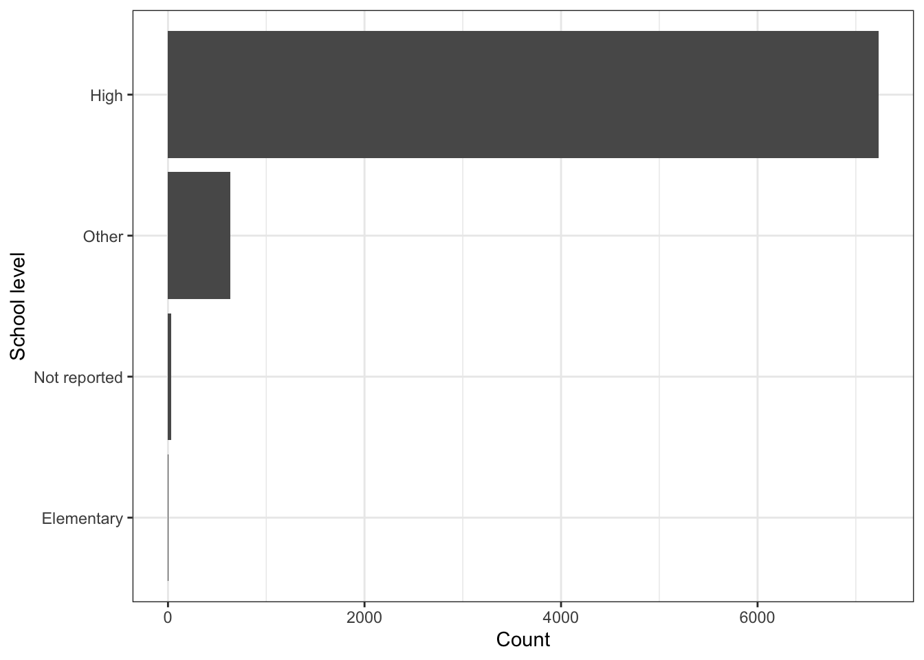
Most of the schools are high schools, but there are some schools listed as Other and Not reported.
It is strange that students in an elementary school are taking the ACT or SAT. We will limit our analysis to high schools.
\(\rightarrow\) Modify the edgap data frame to include only the schools that are high schools.
Show Answer
edgap <- edgap %>%
  filter(school_level == 'High')
edgap %>%
count(school_level) %>%
mutate(proportion = round(n/sum(n),3))## # A tibble: 1 × 3
## school_level n proportion
## <chr> <int> <dbl>
## 1 High 7230 12.4 Exploratory data analysis
We have two main goals when doing exploratory data analysis. The first is that we want to understand the data set more completely. The second goal is to explore relationships between the variables to help guide the modeling process to answer our specific question.
2.4.1 Graphical summaries
Make a pairs plot of the ACT scores and the socioeconomic variables. We will use the ggpairs function from the GGally package.
#It may take a few seconds to produce the plot

edgap %>%
  select(-c(id,state,zip_code,school_type,school_level)) %>%
  ggpairs(lower = list(continuous=wrap("smooth"))) +
  theme_bw()
## plot: [1,1] [=>-----------------------------------------------------------------------------] 3% est: 0s
## plot: [1,2] [===>---------------------------------------------------------------------------] 6% est: 2s
## plot: [1,3] [======>------------------------------------------------------------------------] 8% est: 2s
## plot: [1,4] [========>----------------------------------------------------------------------] 11% est: 3s
## plot: [1,5] [==========>--------------------------------------------------------------------] 14% est: 3s
## plot: [1,6] [============>------------------------------------------------------------------] 17% est: 2s
## plot: [2,1] [==============>----------------------------------------------------------------] 19% est: 2s
## plot: [2,2] [=================>-------------------------------------------------------------] 22% est: 2s
## plot: [2,3] [===================>-----------------------------------------------------------] 25% est: 2s
## plot: [2,4] [=====================>---------------------------------------------------------] 28% est: 2s
## plot: [2,5] [=======================>-------------------------------------------------------] 31% est: 2s
## plot: [2,6] [=========================>-----------------------------------------------------] 33% est: 2s
## plot: [3,1] [============================>--------------------------------------------------] 36% est: 2s
## plot: [3,2] [==============================>------------------------------------------------] 39% est: 2s
## plot: [3,3] [================================>----------------------------------------------] 42% est: 2s
## plot: [3,4] [==================================>--------------------------------------------] 44% est: 2s
## plot: [3,5] [====================================>------------------------------------------] 47% est: 1s
## plot: [3,6] [=======================================>---------------------------------------] 50% est: 1s
## plot: [4,1] [=========================================>-------------------------------------] 53% est: 1s
## plot: [4,2] [===========================================>-----------------------------------] 56% est: 1s
## plot: [4,3] [=============================================>---------------------------------] 58% est: 1s
## plot: [4,4] [===============================================>-------------------------------] 61% est: 1s
## plot: [4,5] [=================================================>-----------------------------] 64% est: 1s
## plot: [4,6] [====================================================>--------------------------] 67% est: 1s
## plot: [5,1] [======================================================>------------------------] 69% est: 1s
## plot: [5,2] [========================================================>----------------------] 72% est: 1s
## plot: [5,3] [==========================================================>--------------------] 75% est: 1s
## plot: [5,4] [============================================================>------------------] 78% est: 1s
## plot: [5,5] [===============================================================>---------------] 81% est: 1s
## plot: [5,6] [=================================================================>-------------] 83% est: 1s
## plot: [6,1] [===================================================================>-----------] 86% est: 0s
## plot: [6,2] [=====================================================================>---------] 89% est: 0s
## plot: [6,3] [=======================================================================>-------] 92% est: 0s
## plot: [6,4] [==========================================================================>----] 94% est: 0s
## plot: [6,5] [============================================================================>--] 97% est: 0s
## plot: [6,6] [===============================================================================]100% est: 0s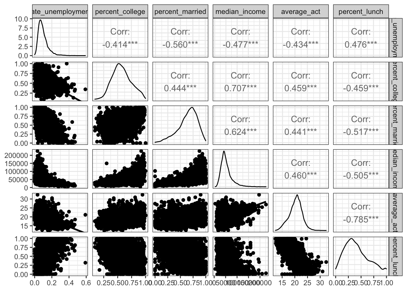
2.4.1.1 Distributions of individual numerical variables
\(\rightarrow\) Describe the shape of the distribution of each variable.
Show Answer
We examine the density plots along the main diagonal of the pairs plots.
All distributions appear to be unimodal.
rate_unemployment has a positively skewed distribution. The values near 0.6 may be outliers.
percent_college has a roughly symmetric distribution.
percent_married has a negatively skewed distribution.
average_act has an approximately normal distribution. This is not surprising for a distribution of averages.
median_income has a positively skewed distribution, which is what you expect for income distributions.
percent_lunch has a slightly positively skewed distribution.
2.4.1.2 Categorical variables
What states are present in the data set and with what frequency?
\(\rightarrow\) First find the states present.Show Answer
edgap %>%
  select(state) %>%
  unique()
## # A tibble: 20 × 1
## state
## <chr>
## 1 DE
## 2 FL
## 3 GA
## 4 IL
## 5 IN
## 6 KY
## 7 LA
## 8 MA
## 9 MI
## 10 MO
## 11 NJ
## 12 NY
## 13 NC
## 14 OH
## 15 PA
## 16 TN
## 17 TX
## 18 WA
## 19 WI
## 20 WY\(\rightarrow\) Now count the observations by state. Display the results as a bar graph.
Show Answer
edgap %>%
  count(state) %>%
  ggplot(aes(x = state, y = n)) +
  geom_col() +
  coord_flip() +
  labs(x = "State", y = "Count") +
  theme_bw()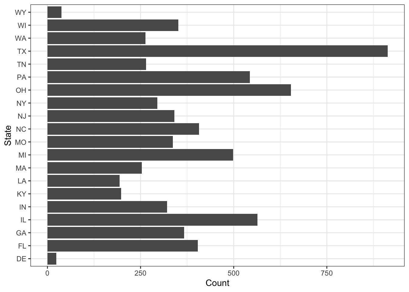
\(\rightarrow\) Reorder the states by count using fct_reorder
Show Answer
edgap %>%
  count(state) %>%
  mutate(state = fct_reorder(state, n)) %>%
  ggplot(aes(x = state, y = n)) +
  geom_col() +
  coord_flip() +
  labs(x = "State", y = "Count") +
  theme_bw()
There is not an equal number of schools from the represented states.
\(\rightarrow\) What school types are present in the data set and with what frequency? Present the results as a table and as a bar graph.
Show Answer
edgap %>%
  count(school_type) %>%
  mutate(proportion = round(n/sum(n),3))
## # A tibble: 4 × 3
## school_type n proportion
## <chr> <int> <dbl>
## 1 Alternative School 9 0.001
## 2 Career and Technical School 1 0
## 3 Regular School 7218 0.998
## 4 Special Education School 2 0The vast majority (99.8%) are regular schools, but there are a few other types of schools.
We can also present the information as a graph:
edgap %>%
count(school_type) %>%
mutate(school_type = fct_reorder(school_type, n)) %>%
ggplot(aes(x = school_type, y = n)) +
geom_col() +
coord_flip() +
labs(x = "School type", y = "Count") +
theme_bw()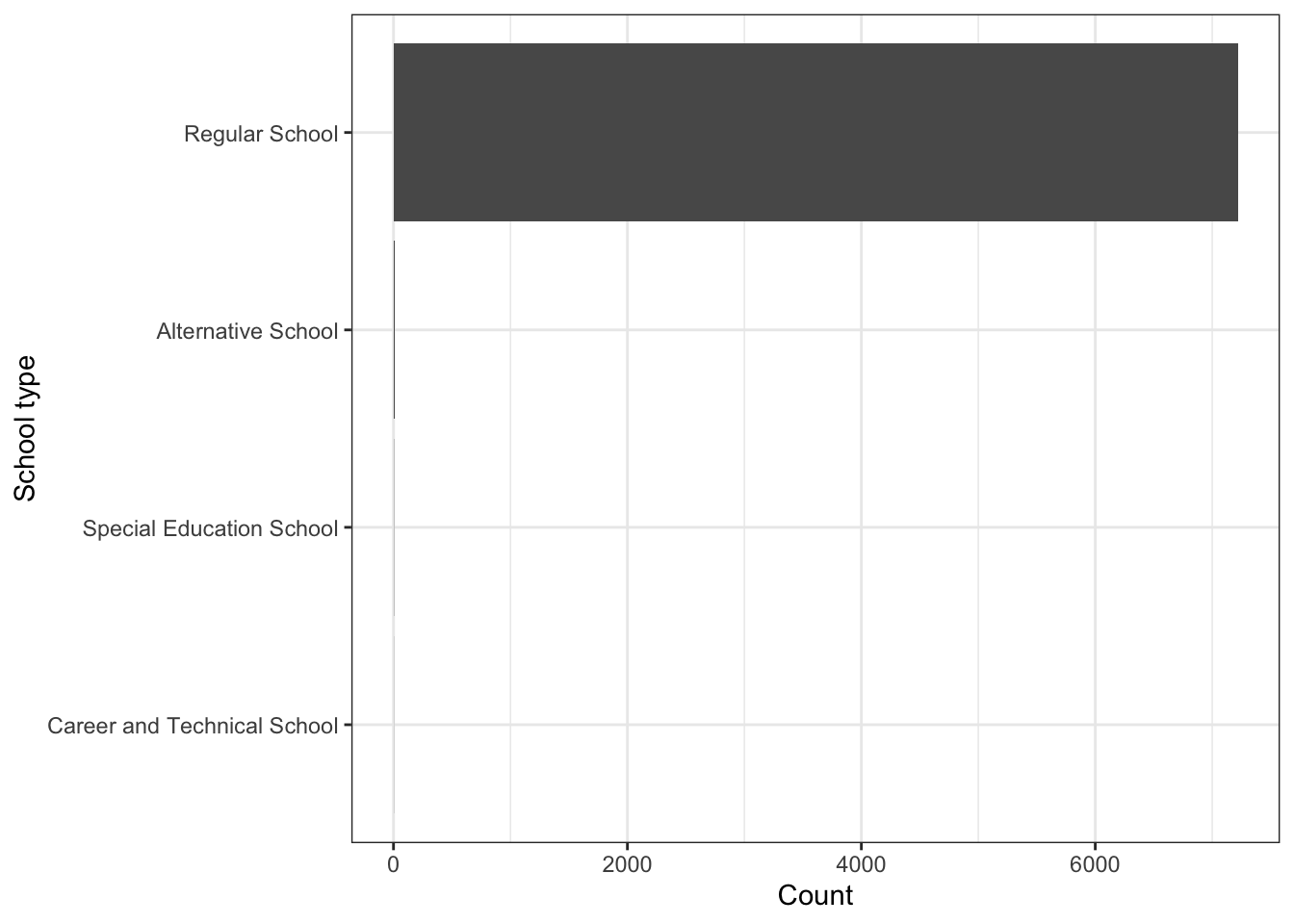 but the graph can be misleading because of the large number of regular schools and the few schools of the other types.
2.4.1.3 Focus on relationships with average_act
Our primary goal is to determine whether there is a relationship between the socioeconomic variables and average_act, so we will make plots to focus on those relationships.
The largest correlation coefficient between a socioeconomic variable and average_act is for percent_lunch, so we will start there.
\(\rightarrow\) Make a scatter plot of percent_lunch and average_act
Show Answer
ggplot(edgap, aes(x = percent_lunch, y = average_act)) +
  geom_point() +
  labs(x = 'Percent reduced or free lunch', y = 'Average school ACT or equivalent if SAT') +
  theme_bw()
## Warning: Removed 23 rows containing missing values (geom_point).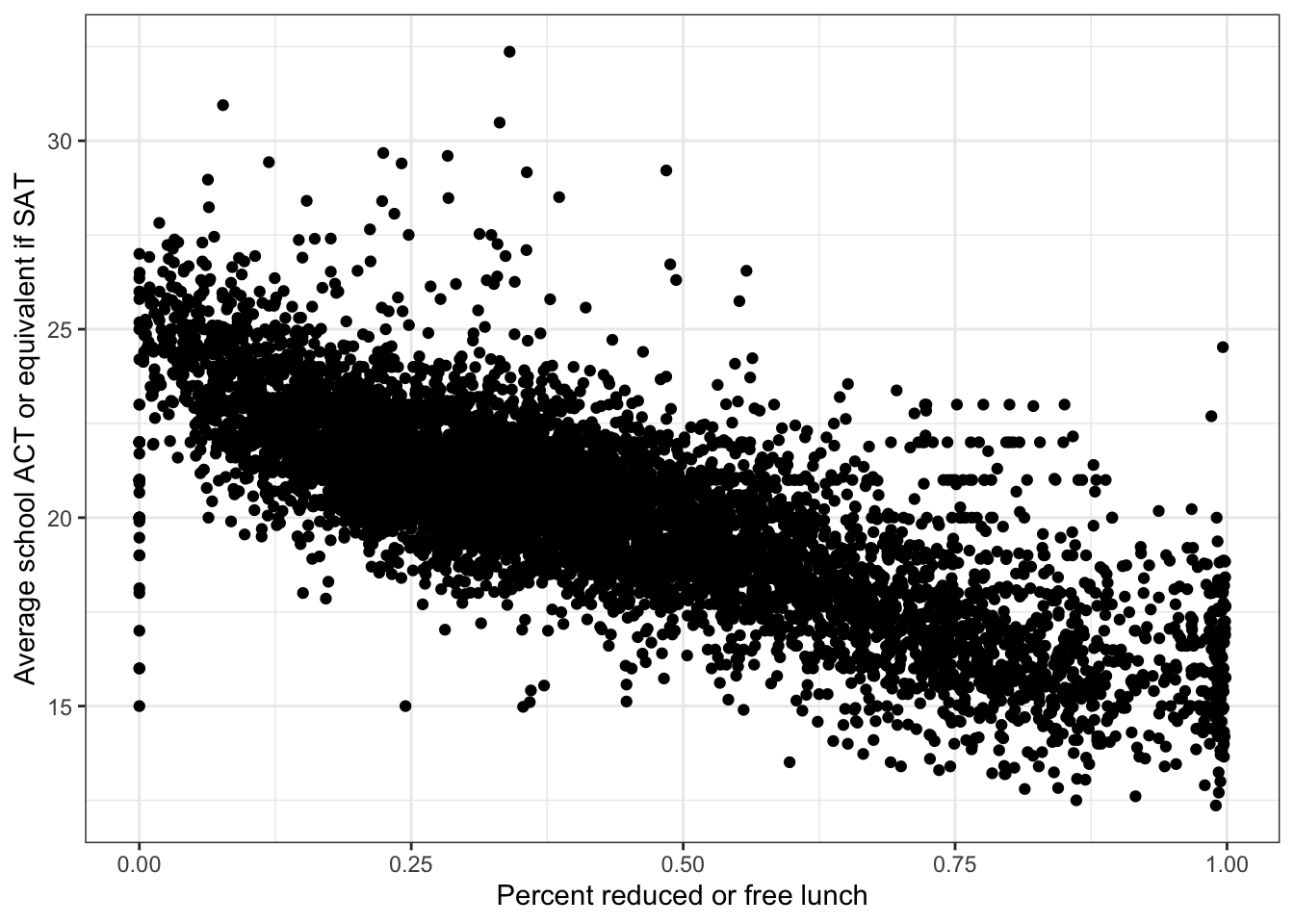
There is a clear negative linear association between percent_lunch and average_act.
Why is there a wide range of ACT scores at percent_lunch = 0? It may be the case that some schools have no students receiving free or reduced lunch because the program does not exist, not because there are no families that would qualify under typical standards. This would require further research into the availability of the free or reduced price lunch program.
\(\rightarrow\) Make a scatter plot of median_income and average_act
Show Answer
ggplot(edgap, aes(x = median_income, y = average_act)) +
  geom_point() +
  labs(x = 'Median income ($)', y = 'Average school ACT or equivalent if SAT' ) +
  theme_bw()
## Warning: Removed 19 rows containing missing values (geom_point).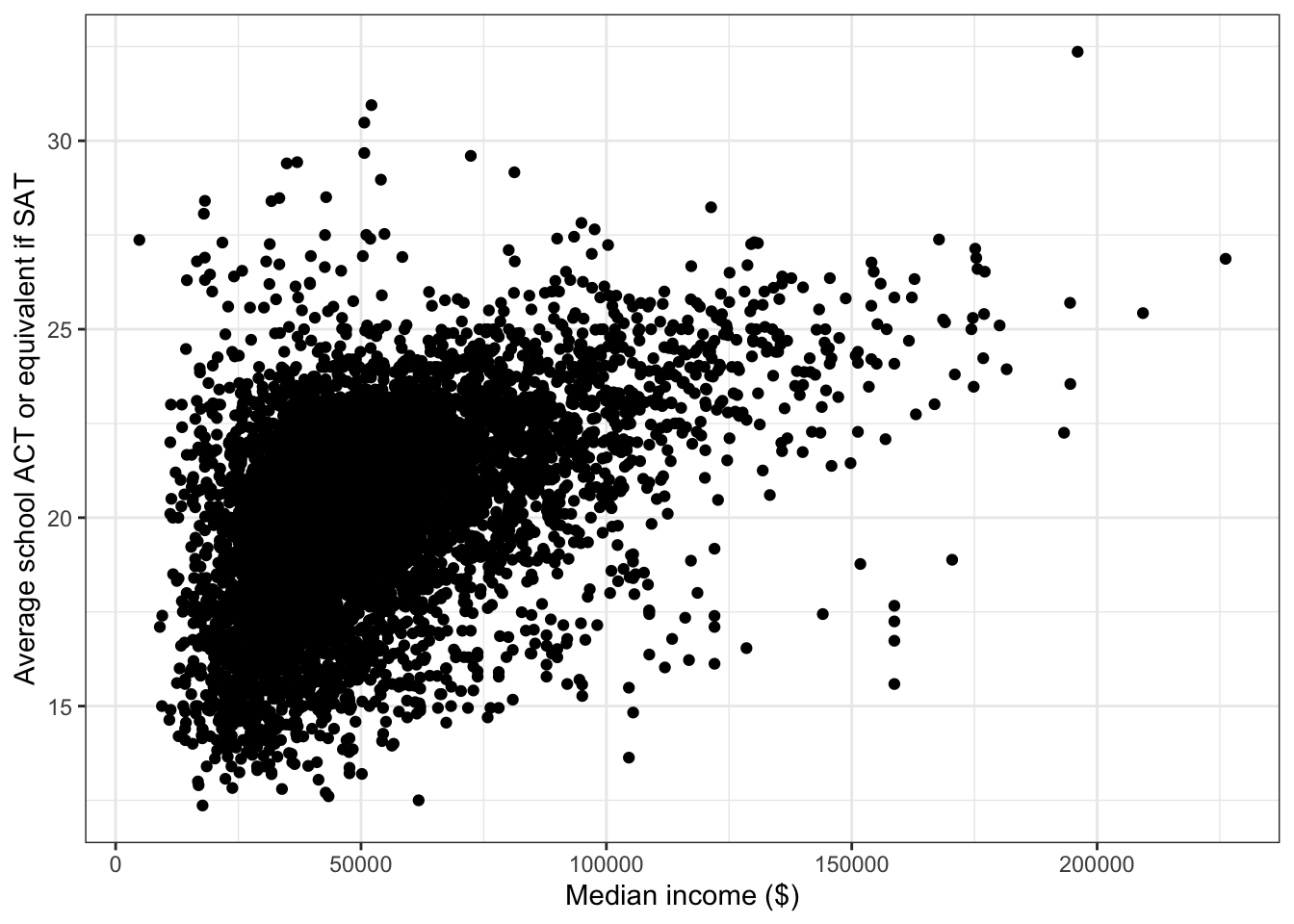
There is a positive association between median_income and average_act. The form of the association appears to be nonlinear.
\(\rightarrow\) median_income has a skewed distribution, so make a scatter plot with median_income plotted on a log scale.
Show Answer
ggplot(edgap, aes(x = median_income, y = average_act)) +
  geom_point() +
  scale_x_log10() +
  labs(x = 'Median income ($)', y = 'Average school ACT or equivalent if SAT' ) +
  theme_bw()
## Warning: Removed 19 rows containing missing values (geom_point).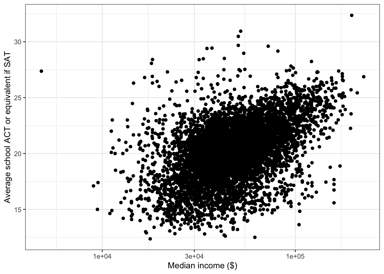
There is a positive linear associate between the log of median_income and average_act. Note also that the typical regression assumption of equal variance of errors is closer to being satisfied after the log transformation.
\(\rightarrow\) Make a scatter plot of percent_college and average_act
Show Answer
ggplot(edgap, aes(x = percent_college, y = average_act)) +
  geom_point() +
  labs(x = 'Percent college', y = 'Average school ACT or equivalent if SAT') +
  theme_bw()
## Warning: Removed 14 rows containing missing values (geom_point).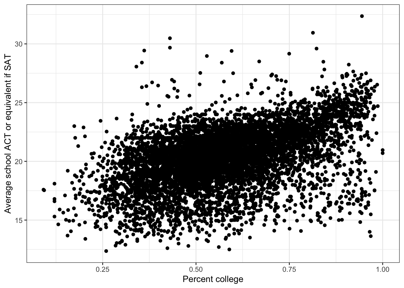
There is a positive association between percent_college and average_act. There may be a nonlinear component to the association, but it is difficult to assess visually from the scatter plot.
\(\rightarrow\) Make a scatter plot of percent_married and average_act
Show Answer
ggplot(edgap, aes(x = percent_married, y = average_act)) +
  geom_point() +
  labs(x = 'Percent college', y = 'Average school ACT or equivalent if SAT') +
  theme_bw()
## Warning: Removed 23 rows containing missing values (geom_point).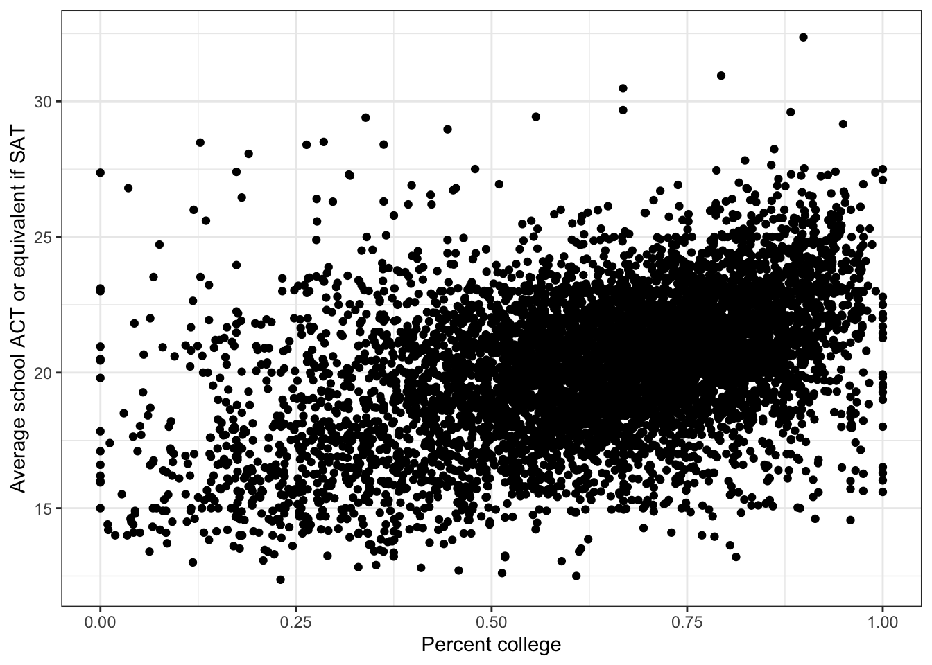
There is a positive association between percent_married and average_act.
\(\rightarrow\) Make a scatter plot of rate_unemployment and average_act
Show Answer
ggplot(edgap, aes(x = rate_unemployment, y = average_act)) +
  geom_point() +
  labs(x = 'Rate of unemployment', y = 'Average school ACT or equivalent if SAT') +
  theme_bw()
## Warning: Removed 15 rows containing missing values (geom_point).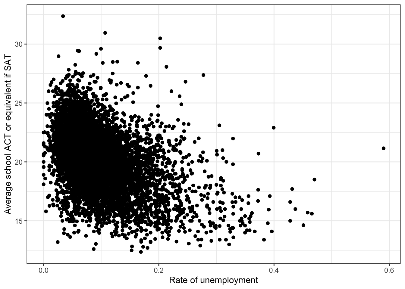 There is a negative association between
 rate_unemployment and average_act.
rate_unemployment has a positively skewed distribution, so we should make a scatter plot on a transformed scale. There are values of rate_unemployment that are equal to zero,
min(edgap$rate_unemployment, na.rm = TRUE)## [1] 0so we will use a square root transformation, rather than a log transformation.
library(latex2exp) #This library is used for LaTex in the axis labels

edgap %>%
  ggplot(aes(x = sqrt(rate_unemployment), y = average_act)) +
  geom_point() +
  labs(x = TeX('$\\sqrt{$Rate of unemployment$}$'), y = 'Average school ACT or equivalent if SAT') +
  theme_bw()
## Warning: Removed 15 rows containing missing values (geom_point).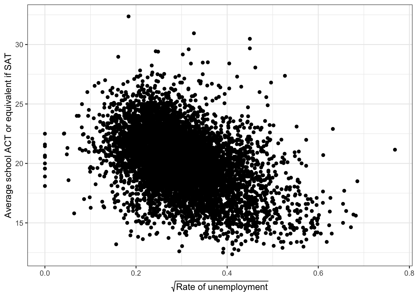
2.4.1.4 Numerical summaries
\(\rightarrow\) Use the skim function to examine the basic numerical summaries for each variable.
Show Answer
edgap %>% select(-id) %>% skim()| Name | Piped data |
| Number of rows | 7230 |
| Number of columns | 10 |
| _______________________ | |
| Column type frequency: | |
| character | 4 |
| numeric | 6 |
| ________________________ | |
| Group variables | None |
Variable type: character
| skim_variable | n_missing | complete_rate | min | max | empty | n_unique | whitespace |
|---|---|---|---|---|---|---|---|
| state | 0 | 1 | 2 | 2 | 0 | 20 | 0 |
| zip_code | 0 | 1 | 5 | 5 | 0 | 6128 | 0 |
| school_type | 0 | 1 | 14 | 27 | 0 | 4 | 0 |
| school_level | 0 | 1 | 4 | 4 | 0 | 1 | 0 |
Variable type: numeric
| skim_variable | n_missing | complete_rate | mean | sd | p0 | p25 | p50 | p75 | p100 | hist |
|---|---|---|---|---|---|---|---|---|---|---|
| rate_unemployment | 12 | 1 | 0.10 | 0.06 | 0.00 | 0.06 | 0.08 | 0.12 | 0.59 | ▇▂▁▁▁ |
| percent_college | 11 | 1 | 0.57 | 0.17 | 0.09 | 0.45 | 0.56 | 0.68 | 1.00 | ▁▅▇▅▂ |
| percent_married | 20 | 1 | 0.64 | 0.19 | 0.00 | 0.53 | 0.67 | 0.78 | 1.00 | ▁▂▅▇▃ |
| median_income | 16 | 1 | 52760.47 | 24365.51 | 4833.00 | 37106.00 | 47404.00 | 62106.00 | 226181.00 | ▇▆▁▁▁ |
| average_act | 3 | 1 | 20.30 | 2.51 | 12.36 | 18.80 | 20.50 | 22.00 | 32.36 | ▁▇▇▁▁ |
| percent_lunch | 20 | 1 | 0.41 | 0.23 | 0.00 | 0.23 | 0.37 | 0.56 | 1.00 | ▅▇▆▃▂ |
2.5 Model
Our exploratory data analysis has led to the following observations that will help guide the modeling process:
- Each of the socioeconomic variables is associated with the ACT score and is worthwhile to consider as a predictor.
- Some of the socioeconomic variables may have a nonlinear relationship with the ACT score, so nonlinear models should be explored.
- The socioeconomic variables are correlated with each other, so the best prediction of ACT score might not include all socioeconomic variables.
2.5.1 Simple linear regression with each socioeconomic predictor
In this project, we are very concerned with understanding the relationships in the data set; we are not only concerned with building a model with the highest prediction accuracy. Therefore, we will start by looking at simple linear regression models using each socioeconomic predictor.
2.5.1.1 Percent free or reduced lunch
Fit a model
We want to fit the simple linear regression model
average_act \(\approx \beta_0 + \beta_1\) percent_lunch
Use the function lm to fit a simple linear regression model.
fit_pl <- lm(average_act ~ percent_lunch, data = edgap)Use the summary function to
- Interpret the coefficients in the model.
- Assess the statistical significance of the coefficient on the predictor variable.
summary(fit_pl)$coefficients## Estimate Std. Error t value Pr(>|t|)
## (Intercept) 23.744781 0.03693874 642.815 0
## percent_lunch -8.393695 0.07814631 -107.410 0The intercept is 23.7 and the slope is -8.39. The intercept is interpreted as the best estimate for the mean ACT score when percent_lunch is zero. The slope can be interpreted as saying that a percent_lunch increase of 0.1 is associated with a decrease in the estimated mean ACT score of -0.839 points.
The slope is highly statistically significant, as the p-values are reported as zero. So, there is a statistically significant relationship between percent_lunch and the average ACT score in a school.
Plot the regression line together with the scatter plot
#geom_smooth(method = "lm",formula = y ~ x) adds the regression line to the scatter plot

ggplot(edgap, aes(x = percent_lunch, y = average_act)) +
  geom_point() +
  geom_smooth(method = "lm",formula = y ~ x) +
  labs(x = "Percent free or reduced lunch", y = "School ACT average (or equivalent if SAT score)") +
  theme_bw()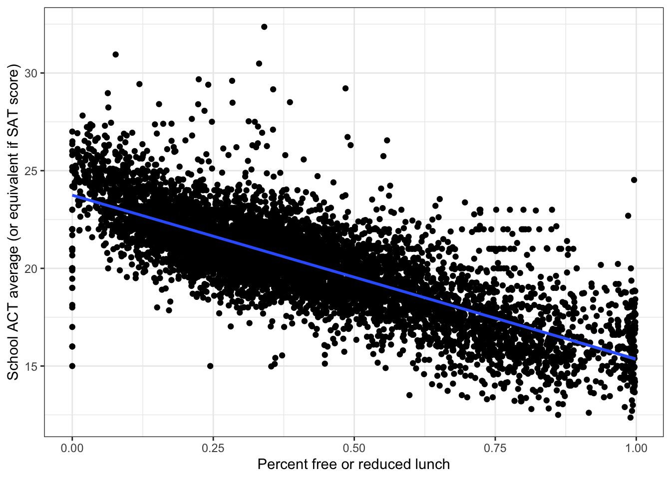
Assess the accuracy of the fit
Examine the \(R^2\) and the residual standard error
summary(fit_pl)$r.squared## [1] 0.6155674The simple linear regression model using percent free or reduced lunch as a predictor can explain 61.6% in the variance of the ACT score.
summary(fit_pl)$sigma## [1] 1.55522The residual standard error is 1.56 points. This means that the model is off by about 1.56 points, on average.
Together, these results show that we can make a good prediction of the average ACT score in a school only by knowing the percent of students receiving free or reduced lunch.
Note that, in this example, we called different components from the summary output individually. We took this approach to walk through each step of the analysis, but you can simply look at the output of summary(fit_pl) to see all of the information at once.
Residual plot
Examine a residual plot to see if we can improve the model through a transformation of the percent_lunch variable.
#We will use ggplot2 to make the residual plot. You can also use plot(fit_pl)
ggplot(fit_pl,aes(x=percent_lunch, y=.resid)) +
  geom_point() +
  geom_smooth(method = "loess", formula = y ~ x) +
  labs(x = "Percent free or reduced lunch", y = "Residuals") +
  theme_bw()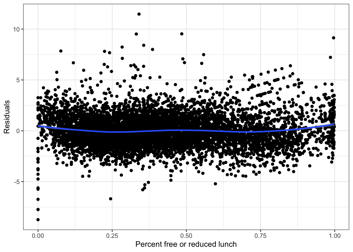
The residual plot does not have much systematic structure, so we have used percent_lunch as well as we can as a predictor. We do not need to consider a more complicated model that only uses percent_lunch as an input variable.
2.5.1.2 Median income
Fit a model
We want to fit the simple linear regression model
average_act \(\approx \beta_0 + \beta_1\) median_income
\(\rightarrow\) Use the function lm to fit a simple linear regression model.
Show Answer
fit_mi <- lm(average_act ~ median_income, data = edgap)\(\rightarrow\) Use the summary function to:
- Interpret the coefficients in the model.
- Assess the statistical significance of the coefficient on the predictor variable.
Show Answer
summary(fit_mi)$coefficients## Estimate Std. Error t value Pr(>|t|)
## (Intercept) 1.780119e+01 6.253060e-02 284.67963 0
## median_income 4.733825e-05 1.075819e-06 44.00205 0The intercept is 17.8 and the slope is \(4.7 \times 10^{-5}\).
The intercept is interpreted as the best estimate for the mean ACT score when median_income is zero. The median income is never equal to zero, so the intercept does not have a clear interpretation in this model.
The slope can be interpreted as saying that a difference of $1 in median_income is associated with a difference in the estimated mean ACT score of \(4.7 \times 10^{-5}\) points. This value of the slope is not intuitive because the median income is in dollars, but differences in annual income of several dollars is not meaningful. It would be helpful to represent median income in tens of thousands of dollars to make a one-unit change more meaningful.
We will use the mutate function to add a new variable to the data frame called median_income_10k that represents median income in tens of thousands of dollars.
edgap <- edgap %>%
  mutate(median_income_10k = median_income/1e4)
We can refit the model
fit_mi <- lm(average_act ~ median_income_10k, data = edgap)

summary(fit_mi)$coefficients
## Estimate Std. Error t value Pr(>|t|)
## (Intercept) 17.8011868 0.06253060 284.67963 0
## median_income_10k 0.4733825 0.01075819 44.00205 0The intercept remains 17.8, but the slope is now 0.47, corresponding to the scaling of the median income units.
The slope can be interpreted as saying that a difference of $10,000 in median income is associated with a difference in the estimated mean ACT score of 0.47 points.
The slope is highly statistically significant. So, there is a statistically significant relationship between median income and the average ACT score in a school.
\(\rightarrow\) Plot the regression line together with the scatter plot
Show Answer
ggplot(edgap, aes(x = median_income_10k, y = average_act)) +
  geom_point() +
  geom_smooth(method = "lm",formula = y ~ x) +
  labs(x = "Median Household Income (ten thousand $)", y = "School ACT average (or equivalent if SAT score)") +
  theme_bw()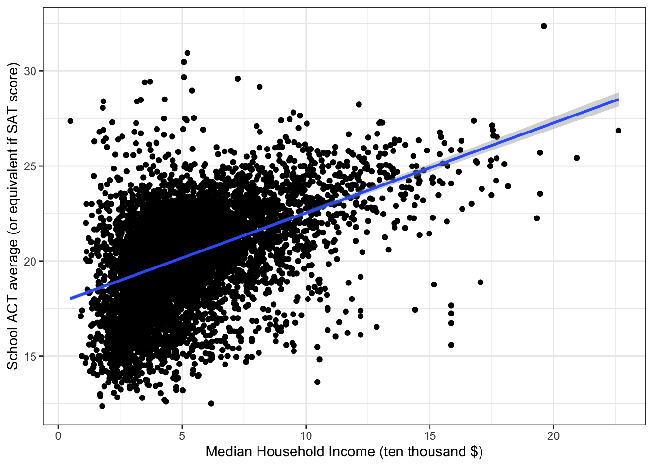
Assess the accuracy of the fit
\(\rightarrow\) Examine the \(R^2\) and the residual standard error
Show Answer
summary(fit_mi)$r.squared## [1] 0.2117159The simple linear regression model using median income as a predictor explains 21.2% in the variance of the ACT score.
summary(fit_mi)$sigma## [1] 2.225708The residual standard error is 2.26 points. This means that the model is off by about 2.26 points, on average.
Together, these results show that we can do some moderate prediction of the average ACT score in a school only by knowing the median income.
Residual plot
\(\rightarrow\) Examine a residual plot to see if we can improve the model through a transformation of the median_income_10 variable.
Show Answer
ggplot(fit_mi,aes(x=median_income_10k, y=.resid)) +
  geom_point() +
  geom_smooth(method = "loess", formula = y ~ x) +
  labs(x = "Median Household Income (ten thousand $)", y = "Residuals") +
  theme_bw()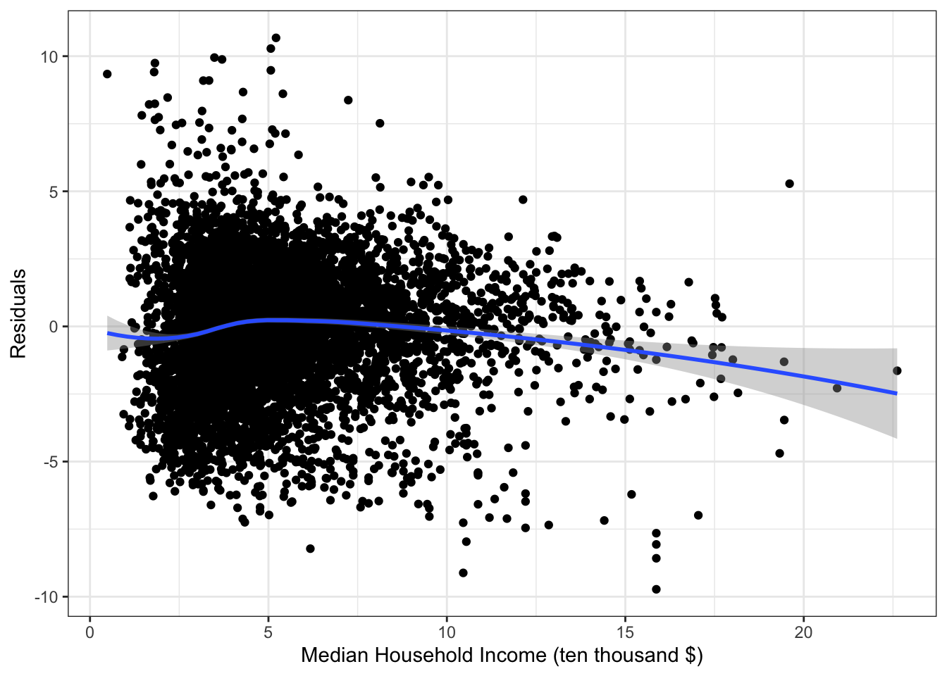
The residual plot suggests that a nonlinear model may improve the fit.
We will try a log transformation.Log transformation
Fit the model
\(\rightarrow\) Fit a linear regression model using the log of median_income_10 as the predictor.
Show Answer
fit_mi_log <- lm(average_act ~ log10(median_income_10k), data = edgap)\(\rightarrow\) Use the summary function to:
- Interpret the coefficients in the model.
- Assess the statistical significance of the coefficient on the predictor variable.
Show Answer
summary(fit_mi_log)$coefficients## Estimate Std. Error t value Pr(>|t|)
## (Intercept) 16.040603 0.09908011 161.89529 0
## log10(median_income_10k) 6.245003 0.14014512 44.56097 0The intercept is 16.0. The intercept is interpreted as the prediction of the average ACT score when the predictor is zero, which means that the median income is $10,000.
The slope is 6.3. Because we used a base 10 log, the slope is interpreted as saying that a median income ten times greater than another is associated with an average ACT score that is 6.3 points higher.
The slope is highly statistically significant.\(\rightarrow\) Plot the regression line together with the scatter plot
Show Answer
ggplot(edgap, aes(x = log10(median_income_10k), y = average_act)) +
  geom_point() +
  geom_smooth(method = "lm",formula = y ~ x) +
  labs(x = "Log of median Household Income", y = "School ACT average (or equivalent if SAT score)") +
  theme_bw()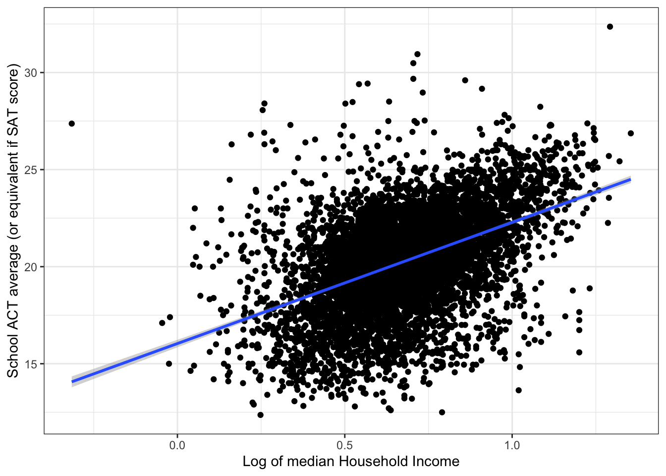
Assess the accuracy of the fit
\(\rightarrow\) Examine the \(R^2\) and the residual standard error
Show Answer
summary(fit_mi_log)$r.squared## [1] 0.2159597The simple linear regression model using median income as a predictor can explain 21.6% in the variance of the ACT score.
summary(fit_mi_log)$sigma## [1] 2.219709The residual standard error is 2.22 points. This means that the model is off by about 2.22 points, on average.
Together, these results show that we can do some moderate prediction of the average ACT score in a school only by knowing the median income.Residual plot
\(\rightarrow\) Examine a residual plot to see if we can improve the model through a transformation of the input.
Show Answer
ggplot(fit_mi_log, aes(x=.fitted, y=.resid)) +
  geom_point() +
  geom_smooth(method = "loess", formula = y ~ x) +
  labs(x = "Log Median Household Income", y = "Residuals") +
  theme_bw()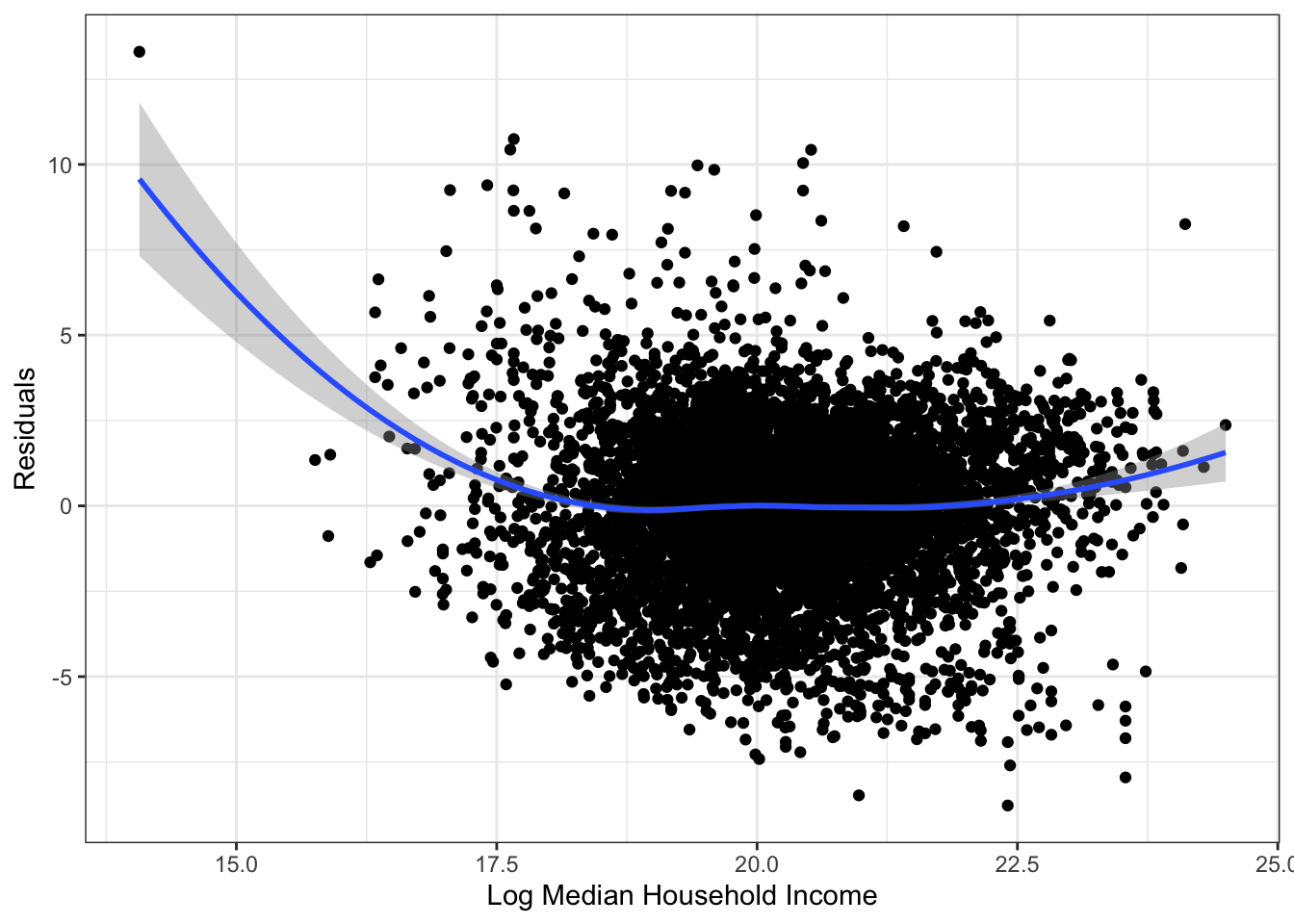
2.5.1.3 Percent college
Fit a model
We want to fit the simple linear regression model
average_act \(\approx \beta_0 + \beta_1\) percent_college
\(\rightarrow\) Use the function lm to fit a simple linear regression model.
Show Answer
fit_pc <- lm(average_act ~ percent_college, data = edgap)\(\rightarrow\) Use the summary function to
- Interpret the coefficients in the model.
- Assess the statistical significance of the coefficient on the predictor variable.
Show Answer
summary(fit_pc)$coefficients## Estimate Std. Error t value Pr(>|t|)
## (Intercept) 16.307759 0.09476034 172.09477 0
## percent_college 6.966002 0.15889860 43.83929 0The slope is highly statistically significant. So, there is a statistically significant relationship between percent college and the average ACT score in a school.
\(\rightarrow\) Plot the regression line together with the scatter plot
Show Answer
ggplot(edgap, aes(x = percent_college, y = average_act)) +
  geom_point() +
  geom_smooth(method = "lm",formula = y ~ x) +
  labs(x = "Percent college", y = "School ACT average (or equivalent if SAT score)") +
  theme_bw()
## Warning: Removed 14 rows containing non-finite values (stat_smooth).## Warning: Removed 14 rows containing missing values (geom_point).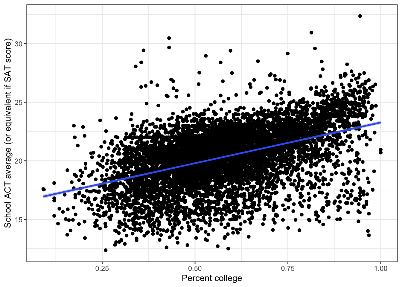
Assess the accuracy of the fit
\(\rightarrow\) Examine the \(R^2\) and the residual standard error
Show Answer
summary(fit_pc)$r.squared## [1] 0.2103665The simple linear regression model using median income as a predictor can explain 21.0% in the variance of the ACT score.
summary(fit_pc)$sigma## [1] 2.227256The residual standard error is 2.23 points. This means that the model is off by about 2.23 points, on average.
Together, these results show that we can do some moderate prediction of the average ACT score in a school only by knowing the percent of college graduates among adults.Residual plot
\(\rightarrow\) Examine a residual plot to see if we can improve the model through a transformation of the input variable.
Show Answer
ggplot(fit_pc, aes(x=percent_college, y=.resid)) +
  geom_point() +
  geom_smooth(method = "loess", formula = y ~ x) +
  labs(x = "Percent college", y = "Residuals") +
  theme_bw()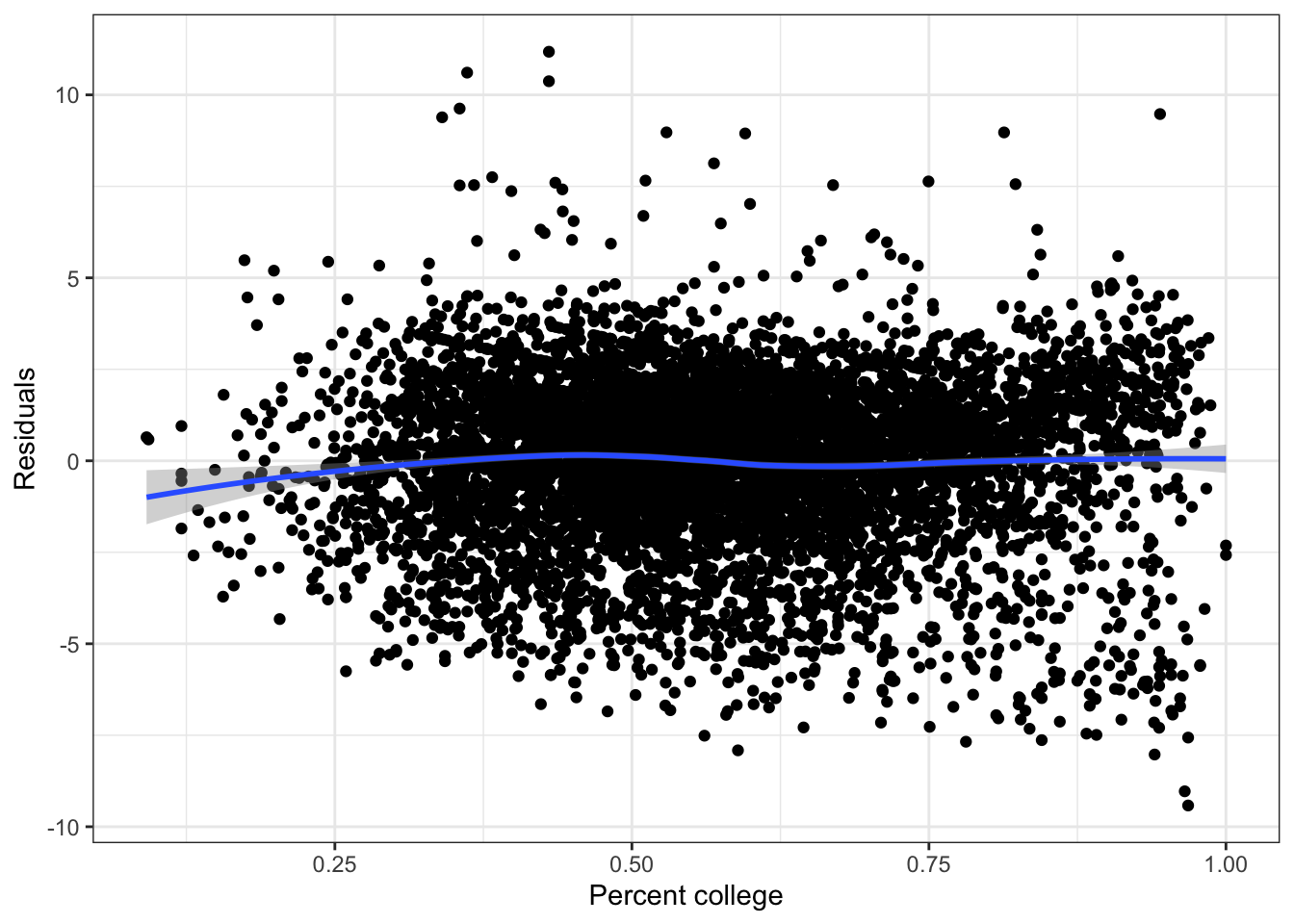
The residual plot has a small suggestion that a quadratic model might be useful.
\(\rightarrow\) Fit and assess a quadratic model
Show Answer
fit_pc_quad <- lm(average_act ~ poly(percent_college,2, raw = T), data = edgap)summary(fit_pc_quad)##
## Call:
## lm(formula = average_act ~ poly(percent_college, 2, raw = T),
## data = edgap)
##
## Residuals:
## Min 1Q Median 3Q Max
## -9.3502 -1.2283 0.2854 1.4668 11.1775
##
## Coefficients:
## Estimate Std. Error t value Pr(>|t|)
## (Intercept) 16.1091 0.2686 59.980 <2e-16 ***
## poly(percent_college, 2, raw = T)1 7.6930 0.9333 8.242 <2e-16 ***
## poly(percent_college, 2, raw = T)2 -0.6129 0.7754 -0.790 0.429
## ---
## Signif. codes: 0 '***' 0.001 '**' 0.01 '*' 0.05 '.' 0.1 ' ' 1
##
## Residual standard error: 2.227 on 7213 degrees of freedom
## (14 observations deleted due to missingness)
## Multiple R-squared: 0.2104, Adjusted R-squared: 0.2102
## F-statistic: 961.2 on 2 and 7213 DF, p-value: < 2.2e-16The coefficient on the squared term is not significant, so the quadratic model does not provide an improvement over the linear model.
2.5.1.4 Rate of unemployment
Fit a model
We want to fit the simple linear regression model
average_act \(\approx \beta_0 + \beta_1\) rate_unemployment
\(\rightarrow\) Use the function lm to fit a simple linear regression model.
Show Answer
fit_ru <- lm(average_act ~ rate_unemployment, data = edgap)\(\rightarrow\) Use the summary function to:
- Interpret the coefficients in the model.
- Assess the statistical significance of the coefficient on the predictor variable.
Show Answer
summary(fit_ru)$coefficients## Estimate Std. Error t value Pr(>|t|)
## (Intercept) 22.15006 0.05252349 421.71719 0
## rate_unemployment -19.19084 0.46971479 -40.85636 0\(\rightarrow\) Plot the regression line together with the scatter plot
Show Answer
ggplot(edgap, aes(x = rate_unemployment, y = average_act)) +
  geom_point() +
  geom_smooth(method = "lm",formula = y ~ x) +
  labs(x = "Unemployment rate", y = "School ACT average (or equivalent if SAT score)") +
  theme_bw()
## Warning: Removed 15 rows containing non-finite values (stat_smooth).## Warning: Removed 15 rows containing missing values (geom_point).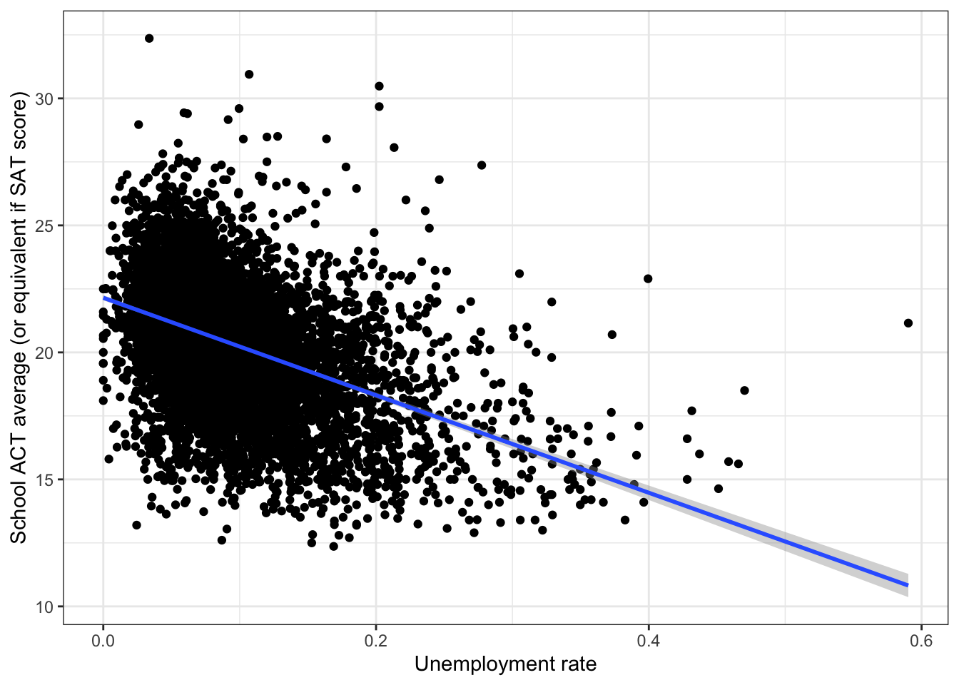
Assess the accuracy of the fit
\(\rightarrow\) Examine the \(R^2\) and the residual standard error
Show Answer
summary(fit_ru)$r.squared## [1] 0.1879303The simple linear regression model using unemployment rate as a predictor can explain 18.8% in the variance of the ACT score.
summary(fit_ru)$sigma## [1] 2.258699The residual standard error is 2.26 points. This means that the model is off by about 2.26 points, on average.
Together, these results show that we can do some moderate prediction of the average ACT score in a school only by knowing the unemployment rate.Residual plot
\(\rightarrow\) Examine a residual plot to see if we can improve the model.
Show Answer
ggplot(fit_ru,aes(x=rate_unemployment, y=.resid)) +
  geom_point() +
  geom_smooth(method = "loess", formula = y ~ x) +
  labs(x = "Unemployment rate", y = "Residuals") +
  theme_bw()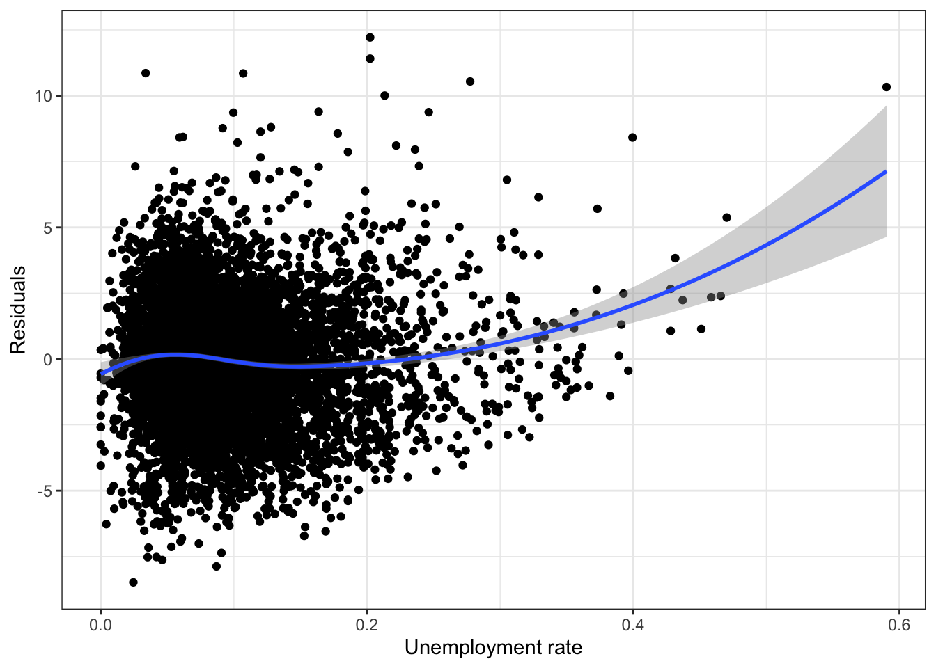
Try a square root transformation of rate_unemployment
Show Answer
fit_ru_sqrt <- lm(average_act ~ sqrt(rate_unemployment), data = edgap)summary(fit_ru_sqrt)##
## Call:
## lm(formula = average_act ~ sqrt(rate_unemployment), data = edgap)
##
## Residuals:
## Min 1Q Median 3Q Max
## -8.9088 -1.3999 0.0888 1.4304 12.1059
##
## Coefficients:
## Estimate Std. Error t value Pr(>|t|)
## (Intercept) 24.09827 0.09705 248.3 <2e-16 ***
## sqrt(rate_unemployment) -12.72070 0.31252 -40.7 <2e-16 ***
## ---
## Signif. codes: 0 '***' 0.001 '**' 0.01 '*' 0.05 '.' 0.1 ' ' 1
##
## Residual standard error: 2.26 on 7213 degrees of freedom
## (15 observations deleted due to missingness)
## Multiple R-squared: 0.1868, Adjusted R-squared: 0.1867
## F-statistic: 1657 on 1 and 7213 DF, p-value: < 2.2e-16The square root transformation provides a small improvement over the linear model.
ggplot(edgap, aes(x = rate_unemployment, y = average_act)) +
  geom_point() +
  geom_smooth(method = "lm", formula = y ~ x) +
  geom_smooth(method = "lm", formula = y ~ sqrt(x),color = 'red') +
  labs(x = "Unemployment rate", y = "School ACT average (or equivalent if SAT score)") +
  theme_bw()
## Warning: Removed 15 rows containing non-finite values (stat_smooth).
## Removed 15 rows containing non-finite values (stat_smooth).## Warning: Removed 15 rows containing missing values (geom_point).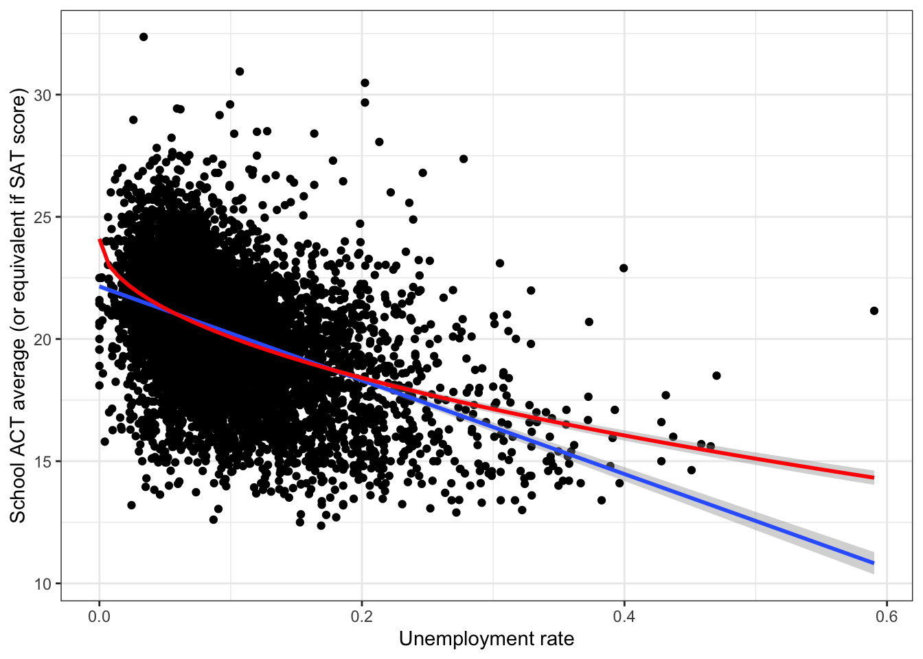
The models are very similar for most of the data, but differ a lot for high unemployment rates. There are few data points with high unemployment rates, so the numerical measures of accuracy are very similar.
ggplot(fit_ru_sqrt,aes(x=.fitted, y=.resid)) +
  geom_point() +
  geom_smooth(method = "loess", formula = y ~ x) +
  labs(x = "Square root of unemployment rate", y = "Residuals") +
  theme_bw()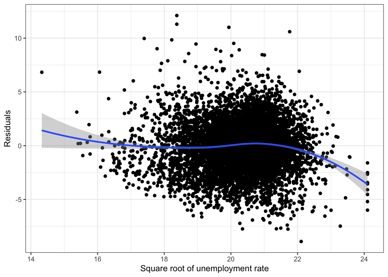
2.5.1.5 Percent married
Fit a model
We want to fit the simple linear regression model
average_act \(\approx \beta_0 + \beta_1\) percent_married
\(\rightarrow\) Use the function lm to fit a simple linear regression model.
Show Answer
fit_pm <- lm(average_act ~ percent_married, data = edgap)\(\rightarrow\) Use the summary function to:
- Interpret the coefficients in the model.
- Assess the statistical significance of the coefficient on the predictor variable.
Show Answer
summary(fit_pm)$coefficients## Estimate Std. Error t value Pr(>|t|)
## (Intercept) 16.599927 0.09268168 179.10690 0
## percent_married 5.774247 0.13862735 41.65301 0\(\rightarrow\) Plot the regression line together with the scatter plot
Show Answer
ggplot(edgap, aes(x = percent_married, y = average_act)) +
  geom_point() +
  geom_smooth(method = "lm",formula = y ~ x) +
  labs(x = "Percent married", y = "School ACT average (or equivalent if SAT score)") +
  theme_bw()
## Warning: Removed 23 rows containing non-finite values (stat_smooth).## Warning: Removed 23 rows containing missing values (geom_point).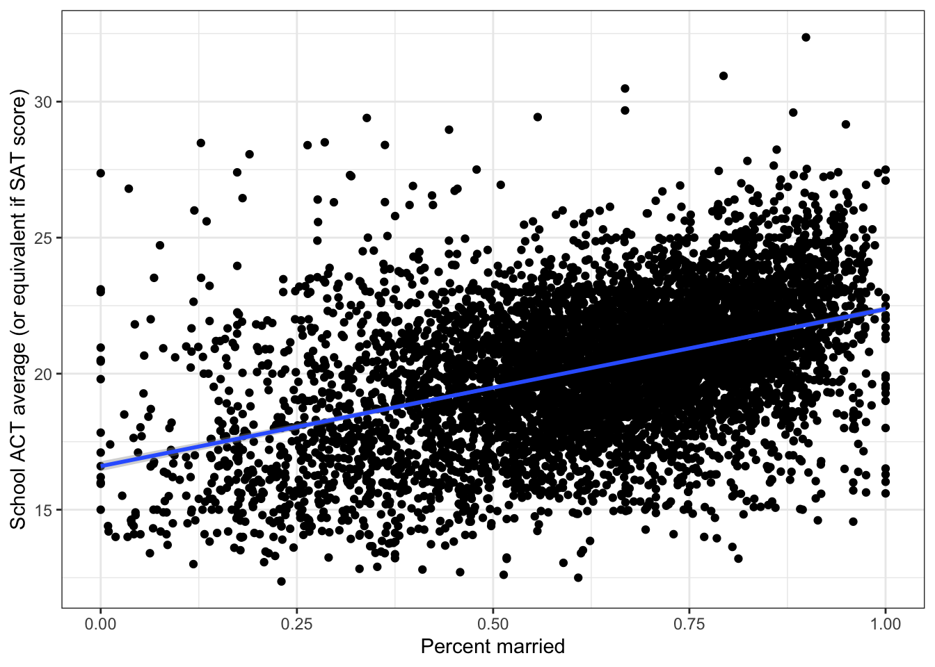
Assess the accuracy of the fit
\(\rightarrow\) Examine the \(R^2\) and the residual standard error
Show Answer
summary(fit_pm)$r.squared## [1] 0.1940692The simple linear regression model using percent married as a predictor can explain 19.4% in the variance of the ACT score.
summary(fit_pm)$sigma## [1] 2.250251The residual standard error is 2.25 points. This means that the model is off by about 2.25 points, on average.
Together, these results show that we can do some moderate prediction of the average ACT score in a school only by knowing the median income.Residual plot
\(\rightarrow\) Examine a residual plot to see if we can improve the model.
Show Answer
ggplot(fit_pm,aes(x=percent_married, y=.resid)) +
  geom_point() +
  geom_smooth(method = "loess", formula = y ~ x) +
  labs(x = "Percent married", y = "Residuals") +
  theme_bw()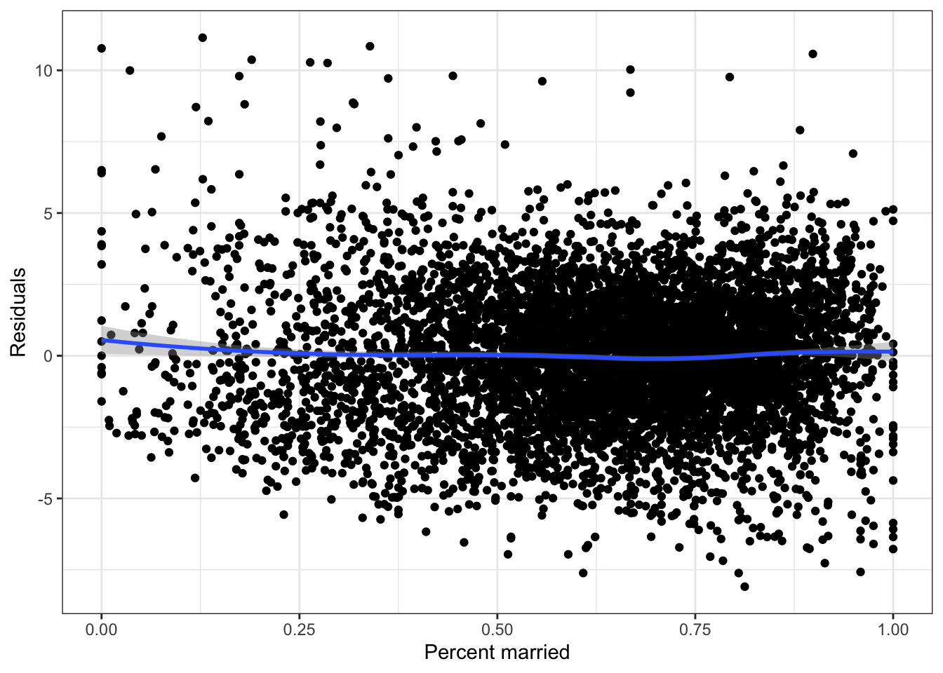
The residual plot suggests a quadratic model may be useful.
fit_pm_quad <- lm(average_act ~ poly(percent_married, 2, raw = T), data = edgap)summary(fit_pm_quad)##
## Call:
## lm(formula = average_act ~ poly(percent_married, 2, raw = T),
## data = edgap)
##
## Residuals:
## Min 1Q Median 3Q Max
## -8.1179 -1.4156 0.0554 1.3895 10.9173
##
## Coefficients:
## Estimate Std. Error t value Pr(>|t|)
## (Intercept) 17.0161 0.1808 94.093 < 2e-16 ***
## poly(percent_married, 2, raw = T)1 4.0920 0.6430 6.364 2.08e-10 ***
## poly(percent_married, 2, raw = T)2 1.4801 0.5524 2.679 0.00739 **
## ---
## Signif. codes: 0 '***' 0.001 '**' 0.01 '*' 0.05 '.' 0.1 ' ' 1
##
## Residual standard error: 2.249 on 7204 degrees of freedom
## (23 observations deleted due to missingness)
## Multiple R-squared: 0.1949, Adjusted R-squared: 0.1946
## F-statistic: 871.8 on 2 and 7204 DF, p-value: < 2.2e-16The quadratic term is statistically significant, even though the improvement in accuracy is not large.
ggplot(edgap, aes(x = percent_married, y = average_act)) +
  geom_point() +
  geom_smooth(method = "lm",formula = y ~ x) +
  geom_smooth(method = "lm",formula = y ~ poly(x,2), color = "red") +
  labs(x = "Percent married", y = "School ACT average (or equivalent if SAT score)") +
  theme_bw()
## Warning: Removed 23 rows containing non-finite values (stat_smooth).
## Removed 23 rows containing non-finite values (stat_smooth).## Warning: Removed 23 rows containing missing values (geom_point).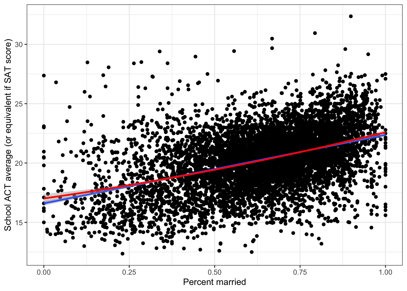
The graph shows that the models are nearly identical.
2.5.2 Model selection
Now that understand how each variable is individually related to the ACT score, we want to know how to best use all of the socioeconomic variables to predict the ACT score.
We do not have many input variables, so we can examine the full model.
fit_full <- lm(average_act ~ percent_lunch + median_income + rate_unemployment + percent_college + percent_married, data = edgap)Examine the summary of the fit
summary(fit_full)##
## Call:
## lm(formula = average_act ~ percent_lunch + median_income + rate_unemployment +
## percent_college + percent_married, data = edgap)
##
## Residuals:
## Min 1Q Median 3Q Max
## -8.5334 -0.9347 -0.0858 0.8578 10.7692
##
## Coefficients:
## Estimate Std. Error t value Pr(>|t|)
## (Intercept) 2.269e+01 1.371e-01 165.492 < 2e-16 ***
## percent_lunch -7.604e+00 9.650e-02 -78.801 < 2e-16 ***
## median_income -1.081e-07 1.205e-06 -0.090 0.929
## rate_unemployment -2.324e+00 4.065e-01 -5.717 1.13e-08 ***
## percent_college 1.754e+00 1.570e-01 11.171 < 2e-16 ***
## percent_married -7.501e-02 1.332e-01 -0.563 0.573
## ---
## Signif. codes: 0 '***' 0.001 '**' 0.01 '*' 0.05 '.' 0.1 ' ' 1
##
## Residual standard error: 1.522 on 7181 degrees of freedom
## (43 observations deleted due to missingness)
## Multiple R-squared: 0.6316, Adjusted R-squared: 0.6314
## F-statistic: 2463 on 5 and 7181 DF, p-value: < 2.2e-16The coefficients for median_income and percent_married are not statistically significant. Additionally, the sign of the coefficients for median_income and percent_married do not make sense. These results support removing median_income and percent_married from the model.
2.5.2.1 Do best subset selection
Use the regsubsets function from the leaps package to perform best subset selection in order to choose the best model to predict average_act from the socioeconomic predictors.
#perform best subset selection
regfit_full <- regsubsets(average_act ~ percent_lunch + median_income + rate_unemployment + percent_college + percent_married, data = edgap)
Get the summary of the best subset selection analysis
reg_summary <- summary(regfit_full)What is the best model obtained according to Cp, BIC, and adjusted \(R^2\)? Make a plot of Cp, BIC, and adjusted \(R^2\) vs. the number of variables in the model.
#Set up a three panel plot
par(mfrow = c(1,3))

#Plot Cp
plot(reg_summary$cp,type = "b",xlab = "Number of variables",ylab = "Cp")
#Identify the minimum Cp
ind_cp = which.min(reg_summary$cp)
points(ind_cp, reg_summary$cp[ind_cp],col = "red",pch = 20)

#Plot BIC
plot(reg_summary$bic,type = "b",xlab = "Number of variables",ylab = "BIC")
#Identify the minimum BIC
ind_bic = which.min(reg_summary$bic)
points(ind_bic, reg_summary$bic[ind_bic],col = "red",pch = 20)

#Plot adjusted R^2
plot(reg_summary$adjr2,type = "b",xlab = "Number of variables",ylab = TeX('Adjusted $R^2$'),ylim = c(0,1))

#Identify the maximum adjusted R^2
ind_adjr2 = which.max(reg_summary$adjr2)
points(ind_adjr2, reg_summary$adjr2[ind_adjr2],col = "red",pch = 20)
The three measures agree that the best model has three variables.
Show the best model for each possible number of variables. Focus on the three variable model.
reg_summary$outmat## percent_lunch median_income rate_unemployment percent_college percent_married
## 1 ( 1 ) "*" " " " " " " " "
## 2 ( 1 ) "*" " " " " "*" " "
## 3 ( 1 ) "*" " " "*" "*" " "
## 4 ( 1 ) "*" " " "*" "*" "*"
## 5 ( 1 ) "*" "*" "*" "*" "*"The best model uses the predictors percent_lunch, rate_unemployment and percent_college.
Fit the best model and examine the results
fit_best <- lm(average_act ~ percent_lunch + rate_unemployment + percent_college, data = edgap)summary(fit_best)##
## Call:
## lm(formula = average_act ~ percent_lunch + rate_unemployment +
## percent_college, data = edgap)
##
## Residuals:
## Min 1Q Median 3Q Max
## -8.4923 -0.9363 -0.0886 0.8611 10.7536
##
## Coefficients:
## Estimate Std. Error t value Pr(>|t|)
## (Intercept) 22.62497 0.10206 221.688 < 2e-16 ***
## percent_lunch -7.59143 0.09212 -82.405 < 2e-16 ***
## rate_unemployment -2.13118 0.37252 -5.721 1.1e-08 ***
## percent_college 1.73653 0.12637 13.741 < 2e-16 ***
## ---
## Signif. codes: 0 '***' 0.001 '**' 0.01 '*' 0.05 '.' 0.1 ' ' 1
##
## Residual standard error: 1.522 on 7191 degrees of freedom
## (35 observations deleted due to missingness)
## Multiple R-squared: 0.6311, Adjusted R-squared: 0.631
## F-statistic: 4101 on 3 and 7191 DF, p-value: < 2.2e-162.5.2.2 Relative importance of predictors
To compare the magnitude of the coefficients, we should first normalize the predictors. Each of the predictors percent_lunch, rate_unemployment and percent_college is limited to the interval (0,1), but they occupy different parts of the interval. We can normalize each variable through a z-score transformation:
scale_z <- function(x, na.rm = TRUE) (x - mean(x, na.rm = na.rm)) / sd(x, na.rm)

edgap_z <- edgap %>%
  mutate_at(c("percent_lunch","rate_unemployment","percent_college"),scale_z)
\(\rightarrow\) Fit the model using the transformed variables and examine the coefficients
Show Answer
fit_z <- lm(average_act ~ percent_lunch + rate_unemployment + percent_college, data = edgap_z)

summary(fit_z)
##
## Call:
## lm(formula = average_act ~ percent_lunch + rate_unemployment +
## percent_college, data = edgap_z)
##
## Residuals:
## Min 1Q Median 3Q Max
## -8.4923 -0.9363 -0.0886 0.8611 10.7536
##
## Coefficients:
## Estimate Std. Error t value Pr(>|t|)
## (Intercept) 20.29713 0.01795 1130.931 < 2e-16 ***
## percent_lunch -1.78055 0.02161 -82.405 < 2e-16 ***
## rate_unemployment -0.12065 0.02109 -5.721 1.1e-08 ***
## percent_college 0.28665 0.02086 13.741 < 2e-16 ***
## ---
## Signif. codes: 0 '***' 0.001 '**' 0.01 '*' 0.05 '.' 0.1 ' ' 1
##
## Residual standard error: 1.522 on 7191 degrees of freedom
## (35 observations deleted due to missingness)
## Multiple R-squared: 0.6311, Adjusted R-squared: 0.631
## F-statistic: 4101 on 3 and 7191 DF, p-value: < 2.2e-16The coefficient on percent_lunch is an order of magnitude larger than the other coefficients. This supports the conclusion that percent_lunch is the most important predictor.
percent_lunch is very close to the performance of the best model.
2.6 Additional step
In addition to completing the above analyses, you should ask and answer one question about the data set. Consult Canvas for further directions.
2.7 Conclusion
After completing your analyses, you will make your conclusions and communicate your results. Consult Canvas for further directions.