2 Data Preparation and Cleaning in R
This chapter will introduce you to viewing, summarizing , and cleaning data following recommendations from the Brief Introduction to the 12 Steps of Data Cleaning (Morrow, 2013).
2.1 Introduction to the Tidyverse
The tidyverse is a set of packages that make R easier to use. All the packages work together and share an underlying grammar and philosophy. That’s right - philosophy. The tidyverse operates on the assumption that data should be “tidy”.
According to Hadley Wickham,Chief Scientist at RStudio and one of the creators of the tidyverse:
Tidy data is a standard way of mapping the meaning of a dataset to its structure. A dataset is messy or tidy depending on how rows, columns and tables are matched up with observations, variables and types. In tidy data:
- Each variable forms a column.
- Each observation forms a row.
- Each type of observational unit forms a table.
You can read more in Tidy Data from the Journal of Statistic Software.
The tidyverse not only helps keep data “tidy,” but makes programming easier compared to the base R syntax. Compare:
2.1.1 Extracting a variable
Tidyverse
select(iris, Species, Petal.Width) # by name
select(iris, 5, 4)  # by column index
Base R
iris[, c("Species", "Petal.Width")] # by name
iris[, c(5, 4)]  # by column index
2.1.2 Make new variables (columns)
Tidyverse
iris %>%
mutate(Petal.Ratio = Petal.Length/Petal.Width,
       Sepal.Ratio = Sepal.Length/Sepal.Width)
Base R
iris$Petal.Ratio <- iris$Petal.Length/iris$Petal.Width
iris$Sepal.Ratio <- iris$Sepal.Length/iris$Sepal.Width
(see more examples here)
Most of this handbook will use tidyverse functions.
2.2 Viewing Your Data
First, let’s load some data. We will be working with R Studio’s “Learning R Survey”.
We will load the data from the URL:
We also added fileEncoding = "UTF-8" to make sure any text was formatted correctly. UTF-8 is a common encoding format.
2.2.1 The RStudio Environment
There are several ways to view this data using the R Studio environment:
- Type the name in the console.
- This is not useful for a large data frame.
- Double-click the data object in the environment.
- This will open up the data frame in the source pane, and you can easily browse the data.
- You can do the same thing using the
view()function, i.e.view(raw_data).
2.2.2 Structure of Data - str()
You can use str() (from base R) to view how your data is structured. That is, whether variables are numeric, characters, factors. If they are factors, you can also see what their levels are. We recommend using str() in the console not your script.
This is a very wide data frame (52 variables/columns), so we will use the following code just to view the structure of the first 5 columns.
## 'data.frame':    1838 obs. of  5 variables:
##  $ Timestamp                                                                                                                                        : chr  "12/13/2019 9:50:30" "12/13/2019 9:50:38" "12/13/2019 9:51:19" "12/13/2019 9:53:51" ...
##  $ How.would.you.rate.your.level.of.experience.using.R.                                                                                             : chr  "Expert" "Beginner" "Intermediate" "Intermediate" ...
##  $ Compared.with.other.technical.topics.you.ve.learned.in.school.and.on.the.job..on.a.scale.of.1.to.5..how.difficult.do.you.expect.learning.R.to.be.: int  NA NA NA NA NA NA NA NA NA NA ...
##  $ From.what.you.know.about.R..how.long.do.you.expect.that.it.will.take.for.you.to.learn.enough.to.use.R.productively.                              : chr  "" "" "" "" ...
##  $ How.do.you.think.you.would.go.about.the.process.of.learning.R.                                                                                   : chr  "" "" "" "" ...
What does the code mean?
str(raw_data)tells R you want to look at the structure of the data object.[1:5]tells R you just want to look at columns 1 to 5
This is what the output means:
Timestampcontains dates but is being read as a factor. Factors are like categories. Multiple data points can share a factor.- This can be converted into a date later using the
lubridatepackage
- This can be converted into a date later using the
How.would.you.rate.your.level.of.experience.using.R.is also a factor. It has 5 levels or categories. “Beginner” is one level. The numbers after the list correspond to the levels of the factors. For example, “Beginner” might be 1 or 2 or 3. We will investigate this more later.Compared.with.other....has the class integer (int). This is a number. The first 10 numbers are all missing (NA).
If you just want to examine a single variable, you can use the $ operator:
## chr [1:1838] "United States of America" "Netherlands" ...In the output, we can see:
Factor- This is a factor (a categorical variable)w/ 93 levels- It has 93 categories (countries)"", "Afghanistan",..:- The first category is "" (i.e. missing), the second category is Afghanistan…and so on, in alphabetical order90 57 90 90 90- These numbers represent the numbers (randomly) assigned to each category.
If you just want to see the class (type) of a variable, you can use the class function:
## [1] "integer"2.2.3 Variable/Column Names - names()
The names() (from base R) function is useful if you just want a list of the variable names.
## [1] "Timestamp"
## [2] "How.would.you.rate.your.level.of.experience.using.R."
## [3] "Compared.with.other.technical.topics.you.ve.learned.in.school.and.on.the.job..on.a.scale.of.1.to.5..how.difficult.do.you.expect.learning.R.to.be."
## [4] "From.what.you.know.about.R..how.long.do.you.expect.that.it.will.take.for.you.to.learn.enough.to.use.R.productively."
## [5] "How.do.you.think.you.would.go.about.the.process.of.learning.R."
2.2.4 First n Rows - head()
The head() (from base R’s utils package) function gives you a slightly more detailed look at your data. It will give you the column name and the first 6 data points (by default):
##             Timestamp
## 1  12/13/2019 9:50:30
## 2  12/13/2019 9:50:38
## 3  12/13/2019 9:51:19
## 4  12/13/2019 9:53:51
## 5 12/13/2019 10:01:03
## 6 12/13/2019 10:04:42
##   How.would.you.rate.your.level.of.experience.using.R.
## 1                                               Expert
## 2                                             Beginner
## 3                                         Intermediate
## 4                                         Intermediate
## 5                                         Intermediate
## 6                                               Expert
You can also request more or less data points per column:
##            Timestamp
## 1 12/13/2019 9:50:30
## 2 12/13/2019 9:50:38
## 3 12/13/2019 9:51:19
##   How.would.you.rate.your.level.of.experience.using.R.
## 1                                               Expert
## 2                                             Beginner
## 3                                         Intermediate
Or you can request data from a single variable using $:
##  [1] 10 10 10  9 10 10  9 10 10 10 10 10 10 10 10 10  9  9  9
## [20]  9
head() looks at the head or top of the data. tail() looks at the bottom:
##  [1]  9 10 10  6 10  6  9 10 10 10  8 10 10 10 10 10  8 NA 10
## [20]  9
2.3 Renaming Variables
If you have noticed, the variable names for the R survey are very long. This is not convenient to work with.
R Studio provides us with a useful code book to help us fix this problem.
A common way of renaming columns is to use the rename() function. This function is part of one of the most useful packages you will download and install: tidyverse.
To begin, install tidyverse: install.packages("tidyverse"). Then load it at the top of your script: library(tidyverse). Don’t forget to run this line of code!
The first column’s name is already simple: Timestamp. So, let’s rename the second column.
First, let’s get the column name (run this in the console because it is part of data exploration and not your script/code):
## [1] "How.would.you.rate.your.level.of.experience.using.R."Now, we can use the rename() function to change this to “Qr_experience”, as listed in the codebook. We will assign this to a new data object for comparison purposes. Put this in your script.
renamed <- raw_data %>%
  rename("Qr_experience" = "How.would.you.rate.your.level.of.experience.using.R.")
Let’s see the new name:
## [1] "Timestamp" "Qr_experience"What does the code mean?
renamed <-creates a new data objectraw_datasays which data object we are working with%>%is the pipe operator. This means something like “and then”rename("new_name" = "old name")sets the name name and the old name. Note the quotation marks
We can read this code like a sentence: Create a data object, “renamed”. Use the “raw_data” object and rename “new_name” from “old_name”.
2.4 Renaming Multiple Variables
We can also rename multiple columns the same way:
renamed <- raw_data %>%
  rename("Qr_experience" = "How.would.you.rate.your.level.of.experience.using.R.",
         "Qr_difficulty_experienced" = "Compared.with.other.technical.topics.you.ve.learned.in.school.and.on.the.job..on.a.scale.of.1.to.5..how.difficult.do.you.expect.learning.R.to.be.")
Let’s check:
## [1] "Qr_experience" "Qr_difficulty_experienced"You can also use names() to change the names of the data frame like this. You can use c to write a list of names and then apply it to the names of your data frame. The names are applied in the order they are written and any missing names are set to NA:
Let’s check:
## [1] "Q1" "Q2"However, raw_data has 52 variables! This would take a long time to do.
Instead of writing 52+ lines of code, we can use the names() function to set the names of our data frame (raw_data) equal to the names of another data frame.
The R Studio survey provides us with a .tsv file of proper variable names for the columns. Let’s load that first:
Let’s use the method above to make a copy of “raw_data” and then rename it:
# make a copy of the data frame
rsurvey <- raw_data

# rename the columns based on qnames
names(rsurvey) <- names(qnames)
Let’s check:
## [1] "Qtime"                "Qr_experience"
## [3] "Qr_difficulty"        "Qr_length_to_success"
Note that renaming follows the order of the “qnames” data frame.
Note also that we named the new data object “rsurvey”. This is the beginning of our clean data set. We don’t want to change anything in our original “raw_data” data frame.
2.5 Cleaning Names with janitor
Let’s make sure all the names are lowercase. This will make typing them in later analyses easier, as you don’t ever need to remember what is capital and what is not. Install the janitor package:
install.packages("janitor")
Run the following code:
Let’s check:
##  [1] "qtime"                  "qr_experience"
##  [3] "qr_difficulty"          "qr_length_to_success"
##  [5] "qhow_to_learn_r"        "qreason_to_learn"
##  [7] "qr_use"                 "qtools"
##  [9] "qobstacles_to_starting" "qr_year"
The clean_names() function will do a number of things:
- convert to lower case
- change spaces into underscores
- change % signs to “percentage”
There are many cool options, so please check ?janitor::clean_names.
2.5.1 Summary Stats - describe()
The psych package offers a very useful function called describe(). This function gives you summary statistics about your data. In particular, it will give you:
- item name
- item number
- number of valid cases
- mean
- standard deviation
- trimmed mean (with trim defaulting to .1)
- median (standard or interpolated
- mad: median absolute deviation (from the median).
- minimum
- maximum
- skew
- kurtosis
- standard error
Install the psych package and load it at the top of your script using library(psych).
The following command describes the first five variables. Note that summary statistics are only given for “qr_difficulty” because, according to str(qr_difficulty), that variable is numeric. The others are categorical and thus are not summarized.
##                       vars    n   mean     sd median trimmed
## qtime*                   1 1838 913.24 526.89  912.5  913.05
## qr_experience*           2 1838   3.41   0.78    4.0    3.53
## qr_difficulty            3    8   3.50   0.53    3.5    3.50
## qr_length_to_success*    4 1838   1.01   0.12    1.0    1.00
## qhow_to_learn_r*         5 1838   1.01   0.13    1.0    1.00
##                          mad min  max range  skew kurtosis
## qtime*                676.07   1 1827  1826  0.00    -1.20
## qr_experience*          0.00   1    5     4 -1.02     0.21
## qr_difficulty           0.74   3    4     1  0.00    -2.23
## qr_length_to_success*   0.00   1    4     3 20.39   456.26
## qhow_to_learn_r*        0.00   1    4     3 19.22   399.20
##                          se
## qtime*                12.29
## qr_experience*         0.02
## qr_difficulty          0.19
## qr_length_to_success*  0.00
## qhow_to_learn_r*       0.00
See more options using ?describe.
2.5.2 Summary Stats - describeBy()
The psych package also provides describeBy (note the capital “B”) to break an integer variable down by some factor or category. For example, the survey provides “qyear_born”, which we can use to calculate age. Then, we can see summary stats of age by experience) from “qr_experience”.
#create an age variable
rsurvey$age <- 2020-rsurvey$qyear_born

#Describe experience by age
describeBy(rsurvey$age, group=rsurvey$qr_experience, mat=TRUE)
## item group1 vars n mean sd median
## X11 1 1 0 NaN NA NA
## X12 2 Beginner 1 224 36.26786 12.968732 34
## X13 3 Expert 1 506 36.62648 9.625914 35
## X14 4 Intermediate 1 993 36.62034 10.948554 35
## X15 5 None 1 8 44.12500 13.798939 42
## trimmed mad min max range skew kurtosis
## X11 NaN NA Inf -Inf -Inf NA NA
## X12 34.76111 11.8608 19 122 103 1.9371531 8.039461
## X13 35.35468 7.4130 22 123 101 2.3352574 13.003583
## X14 35.29560 8.8956 20 142 122 2.1278872 11.839006
## X15 44.12500 12.6021 20 65 45 -0.1578919 -1.082360
## se
## X11 NA
## X12 0.8665099
## X13 0.4279241
## X14 0.3474419
## X15 4.8786616What does the code mean?
rsurvey$age <-- Assign whatever is after the<-to a new column, “age” in “rsurvey”2020-rsurvey$qyear_born- Subtract rsurvey$qyear_born from the current year, 2020.describeBy(age$age,- The numeric variablegroup=age$qr_experience- The grouping variablemat=TRUE)- Show a matrix in the output instead of a more complicated list
2.5.3 Summary Stats - summary()
The summary() function will give similar statistics as describe(), though with less detail. For factors, it will produce a count per level (category). For integers it will produce min, max, quartiles, median, mean, and number of missing data points.
The following summary() function calls columns 2 and 3.
##  qr_experience      qr_difficulty
##  Length:1838        Min.   :3.0
##  Class :character   1st Qu.:3.0
##  Mode  :character   Median :3.5
##                     Mean   :3.5
##                     3rd Qu.:4.0
##                     Max.   :4.0
##                     NA's   :1830
Although both should be factors, “qr_experience” is treated simply as a character class and “qr_difficulty” is treated as numeric. To fix this, you can make changes to the data frame or simply run each variable like this:
##                  Beginner       Expert Intermediate
##           31          233          529         1037
##         None
## 8## 3 4 NA's
## 4 4 18302.5.4 Summary Stats - skim()
skim is another function that produces summary statistics. It will also produce a small histogram to show the distribution of your data (for numeric/integers).
First, install (install.packages("skimr")) skimr
Then, we can use the skim() function like this:
| Name | rsurvey[2:3] |
| Number of rows | 1838 |
| Number of columns | 2 |
| _______________________ | |
| Column type frequency: | |
| character | 1 |
| numeric | 1 |
| ________________________ | |
| Group variables | None |
Variable type: character
| skim_variable | n_missing | complete_rate | min | max | empty | n_unique | whitespace |
|---|---|---|---|---|---|---|---|
| qr_experience | 0 | 1 | 0 | 12 | 31 | 5 | 0 |
Variable type: numeric
| skim_variable | n_missing | complete_rate | mean | sd | p0 | p25 | p50 | p75 | p100 | hist |
|---|---|---|---|---|---|---|---|---|---|---|
| qr_difficulty | 1830 | 0 | 3.5 | 0.53 | 3 | 3 | 3.5 | 4 | 4 | ▇▁▁▁▇ |
2.5.5 Crosstabs - table()
Base R provides the table() function to allow you to view a crosstabulation count of one variable by one or more other variables
We can use the code below to get a list of experience levels by country:
##
##                  Beginner Expert Intermediate None
##               31       18     33           66    0
##   Afghanistan  0        0      0            1    0
##   Albania      0        0      0            1    0
##   Algeria      0        7      5           13    1
##   Andorra      0        0      1            1    0
A Note about
[ ]In the example above, [1:5,] was used. This tells R to take the crosstabs table and look at rows 1:5. Otherwise, there would have been nearly 100 rows of data printed.
[]can be used to refer to a specific rows and columns. It specifies a column index. It is used like this:
data[1]- gets the first columndata[1:5]- gets columns 1 to 5data[1,]- gets the first rowdata[1:5,]- gets rows 1 to 5data[1,1]- gets the first row and first columndata[1:5,1:5]- gets the first five rows and the first five columns
2.6 Keeping and Dropping Variables
We can use select() from tidyverse’s dplyr package to keep specific variables or drop other variables.
Keeping variables:
To drop variables, use the minus sign.
For multiple variables, you can use commas for single columns and colons for a range of columns:
Note that select also places variables in the order specificed.
Alternatively, you can do the same in base R with subset:
keep <- subset(rsurvey, select = qr_experience)
dropped <- subset(rsurvey, select = -qr_experience)
select has more advanced functions such as select_if and select_at. See ?select or ?select_if for more information.
2.7 Keeping and Dropping Rows
Whereas select() works on columns, slice() works on rows:
slice(1:100)keeps rows 1 to 100slice(-1:-100)removes rows 1 to 100slice(1)keeps just row 1slice(-1)removes just row 1
2.8 More Frequencies and Descriptives
You can use any of the following functions to get frequencies of your data:
summary()describe()from thepsychpackageskim()from theskimrpackage
Let’s use the jmv package the get some frequencies:
install.packages("jmv")
We will use the descriptives() function. This will provide nice output. We will use the parameter freq=TRUE to get frequencies for factors.
##
##  DESCRIPTIVES
##
##  Descriptives
##  ----------------------------------------
##               qr_experience    qr_year
##  ----------------------------------------
##    N                   1838        1676
##    Missing                0         162
##    Mean                        2007.749
##    Median                      2015.000
##    Minimum                            2
##    Maximum                         2019
##  ----------------------------------------
##
##
##  FREQUENCIES
##
##  Frequencies of qr_experience
##  --------------------------------------------------------
##    Levels          Counts    % of Total    Cumulative %
##  --------------------------------------------------------
##                                 0.00000         0.00000
##    Beginner           233      12.67682         0.00000
##    Expert             529      28.78128         0.00000
##    Intermediate      1037      56.42002         0.00000
##    None                 8       0.43526         0.00000
##  --------------------------------------------------------
2.9 Spotting Coding Mistakes
You may have noticed that the descriptives for “qr_year” had a minimum of 2. The question reads “What year did you first start learning R?”. This should only contain year data. By running frequencies, you can spot such errors. Let’s take a closer look.
Let’s start by viewing all the data in this question. Since it is year data, let’s arrange it from smallest to greatest and look at the first 10 observations.
##    qr_year
## 1        2
## 2        6
## 3       13
## 4       18
## 5      207
## 6     1977
## 7     1985
## 8     1989
## 9     1989
## 10    1990
Let’s review what we did in the code:
rsurvey %>%tells R to use “rsurvey” and…select(qr_year) %>%select the “qr_year” variable and…arrange(qr_year) %>%arrange the data based on the “qr_year” variable and…head(n = 10)get the first 10 responses.
From the results, we saw that the first 5 responses are invalid years.
2.10 Modifying Data - mutate()
We have a variable, “qr_year” with five invalid cases. They should be years, but are some other numbers. Let’s change those to mising observations using mutate() from the tidyverse.mutate()` allows us to change and create variables (literally mutate the data).
#run this to change the variable
rsurvey <- rsurvey %>%
  mutate(qr_year2 = ifelse(qr_year < 1977, NA, qr_year))

#run this to check
rsurvey %>%
  select(qr_year, qr_year2) %>%
  arrange(qr_year) %>%
  head(n=10)
## qr_year qr_year2
## 1 2 NA
## 2 6 NA
## 3 13 NA
## 4 18 NA
## 5 207 NA
## 6 1977 1977
## 7 1985 1985
## 8 1989 1989
## 9 1989 1989
## 10 1990 1990What does the code mean?
rsurvey <-means we will save our fixed data to the “rsurvey” data object. Essentially, we are overwriting the data object that already exists.rsurvey %>%tells R to use “rsurvey” and…mutate(qr_year2create a new variable, “qr_year2”=which is equal to the following commandifelse(qr_year < 1977, NA, qr_year))if qr_year is less than 1977, write NA, otherwise (else), write the year from qr_year
ifelseis a conditional statement that says:ifelse(if this condition is true, then do this, otherwise do this).
2.11 Reordering Categories - factor()
Many of the factors (categories) in our R survey dataset have been coded to a numeric value, automatically. However, this does not mean the mapping of the number to the factor is correct.
Let’s run this code in the console to check. Since we are just checking, we don’t really want to include this in our script, so we can do basic exploration in the console.
##   qr_experience    n
## 1                 31
## 2      Beginner  233
## 3        Expert  529
## 4  Intermediate 1037
## 5          None    8
You will see that 1 = "“, which is missing data, 2 =”Beginner“, 3 =”Expert“, 4 =”Intermediate" and 5 = “None”. If we were doing a statistical analysis without modifying our data, our results would be severely inaccurate.
Let’s recode this data. We will just do one variable as an example.
recoded <- rsurvey %>%
  select(qr_experience) %>%
  mutate(qr_experience2 = factor(qr_experience,
        levels=c("None","Beginner", "Intermediate", "Expert", NA ))
  )
Let’s check if we are correct. You can run this in the console:
##   qr_experience2    n
## 1           None    8
## 2       Beginner  233
## 3   Intermediate 1037
## 4         Expert  529
## 5           <NA>   31
Now our factors are in the correct order and if we wanted to do some statistical test, it would be much more accurate.
What does the code mean?
recoded <-creates a new data object. We could have overwritten our previous object, but this is to show you the result of recoding.rsurvey %>%tells R to use the “rsurvey” data object and…select(qr_experience) %>%means we are only going to keep this variable in our data (to make demonstration easier), andmutate(means we are going to make a changeqr_experience2 =we will create a new variable “qr_experience2” equal to the next command- Note: we could have done
mutate(qr_experience)and overwritten our column, but if we create a new variable, we can compare them side by side (for demonstration purposes)factor(qr_experience,make a factor from “qr_experience”levels=c("None","Beginner", "Intermediate", "Expert", NA ))set the level names and orders to these.- Note that
NArefers to missing data and is not in quotes)this final parentheses closes themutatefunction. If you place your cursor after it, the corresponding opening parentheses will be highlighted. This is an easy way to check that you have closed all functions, useful for debugging problems. )
This works, so lets apply it to the real data set:
2.12 Clearing Whitespace in Text - str_trim()
On the Learning R survey, there was a question about what industry people were in. This resulted in 135 different responses. However, many of these can be combined to make several large groups. First, let’s view the jobs. To save space, only the first 10 are shown.
##                          qindustry  n
## 1                                  44
## 2                         Academia  2
## 3  Accommodation and Food Services 12
## 4                      Advertising  1
## 5                        Aerospace  1
## 6                       Aerospace   1
## 7                      Agriculture  4
## 8                     Agriculture   1
## 9   Agriculture and animal science  1
## 10                       Agrifood   1
The count() function counts unique values. However, you will notice that many are repeated. That is likely due to random whitespace in or around the text entries. We can use several different functions from tidyverse’s stringr package to fix this.
stringr is loaded when the tidyverse is loaded, so we don’t need to load another library.
str_trim() removes whitespace from the start and end of a string. Let’s also use make sure everything is lowercase using either base R’s tolower() or stringr’s str_to_lower(). They both do the same thing. You can also use str_squish to remove all white space within a string.
Let’s check. You can type this in the console.
##                          qindustry  n
## 1                                  44
## 2                         academia  2
## 3  accommodation and food services 12
## 4                      advertising  1
## 5                        aerospace  2
## 6                      agriculture  5
## 7   agriculture and animal science  1
## 8                         agrifood  1
## 9     analytics consulting company  1
## 10                             any  1
This reduced the number of unique values to 125. That is not ideal, but we have a few more tools we can use to fix this.
First, what does the code mean?
rsurvey <-- saves the following commands to the “rsurvey” data objectrsurvey %>%- means to use the “rsurvey” data object “and then”mutate(- change the dataqindustry =- make the column “qindustry” equal to the followingstr_squish(- trim the whitespace in the following stringtolower(qindustry)))- make the string lowercase and close all parentheses
A Note about Parentheses ( )
In R, it can be easy to become lost with your open and closing parentheses. RStudio provides parenthesese highlighting. Place your cursor on the right side of any parentheses (open or close) and it will highlight to corresponding one. This is a quick way to debug a common problem.
2.13 Combining Categories - case_when()
Looking through the list of jobs, there are some clear categories that we can combine jobs into. For example, agriculture, agriculture and anaimal science, and agrifood can all be combine into an “agriculture” category. We will use three functions to do this:
mutate()to change or create new variablescase_when()as a kind of if/else commandstr_detect()to select specified text
# combine into "agriculture"
rsurvey <- rsurvey %>%
  mutate(
    industry = case_when(
      str_detect(qindustry, "agri") ~ "agriculture",
      TRUE ~ qindustry
    ))

# and check total number
rsurvey %>%
  select(industry) %>%
  distinct() %>% #this line removes duplicates
  count()
## n
## 1 123We now have 123 rows. Let’s see what we did, and then expand it:
What does the code mean?
rsurvey <-- assign to the “rsurvey” objectrsurvey %>%- use “rsurvey” and thenmutate(- change or create a variableindustry = case_when(- create the variable “industry” whenstr_detect(qindustry, "agri")- R detects “agri” in the “qindustry” columns"~ "agriculture",- and rename them “agriculture”TRUE ~ qindustry- everything else is named the name they have in “qindustry”))closes our functions
Let’s expand this to categorize as much as possible. To do this efficiently, We will run rsurvey$industry in the console and scroll through it as we create categories
# combine into "agriculture"
rsurvey <- rsurvey %>%
  mutate(
    industry = case_when(
      str_detect(qindustry, "agri") ~ "agriculture",
      str_detect(qindustry, "health") ~ "health",
      str_detect(qindustry, "education|academia|university|research") ~ "education and research",
      str_detect(qindustry, "marketing|business|trade|ecommerce") ~ "business",
      str_detect(qindustry, "information|analytics|software|cybersecurity|digital|telec") ~ "information technologies",
      str_detect(qindustry, "envi|forest|geo|natural|wildlife|sustain") ~ "environment",
      str_detect(qindustry, "law|legal") ~ "law",
      str_detect(qindustry, "media|journalism") ~ "media",
      str_detect(qindustry, "profit|") ~ "non-profit",
      TRUE ~ "other"
    )
  )

# and check
rsurvey %>% count(industry)
## industry n
## 1 agriculture 7
## 2 business 133
## 3 education and research 704
## 4 environment 33
## 5 health 184
## 6 information technologies 196
## 7 law 4
## 8 media 12
## 9 non-profit 565This code got our data down to 9 categories. The categories are neither perfect nor exhaustive, but they are functional. This is a lesson in working with open-ended data on surveys. A question like this should really have limited options, otherwise, there is a lot to clean!
A Note About Spacing and Tabs
You may have noticed that in the code above,
mutate()was on its own line and there were two parentheses also on their own line. You may have also noticedmutate()was indented as wasstr_detect(). These are not required for the code to function, but are useful to keep the code organized.It is recommend to start a new function after the %>% pipe operator on a new line. It is also recommended to create a new line after a parentheses if it will contain multiple or long arguments.
What did we do differently in the code above?
"law|legal"- You will notice we used the | pipe symbol. This stands for “or”. This command means to look for “law” or “legal”."envi|forest|geo|natural|wildlife|sustain"- You will notice we did not use complete words.str_detect()looks for patterns of string and does not need the complete words unless there are many similar string.- This means “envi” could look for environment, environments, or environmental.
TRUE ~ "other"- We set everything else to the “other” category.
2.14 Splitting variables with split()
The Learning R survey contained a few check-all question types. Depending on the survey platform, these questions either create a new column for each choice or combine all choices in a single column. The Learning R survey did the latter. For example, the question “What applications do you use R for most? (check all that apply)” for the variable “qused_for” looks like this:
## [1] "Statistical analysis, Data transformation, Modeling, Visualization, Machine learning, Text processing"
## [2] "Statistical analysis, Data transformation, Visualization"
## [3] "Statistical analysis, Data transformation, Visualization"
## [4] "Data transformation"
## [5] "Statistical analysis, Data transformation, Modeling, Visualization"
## [6] "Statistical analysis, Data transformation, Modeling, Visualization, Machine learning, Text processing"
How can we work with this type of data? The first thing we can do is split the data so that choices are separated into columns. There are several functions we can use to do this. Normally, we can do this with separate() from tidyverse’s tidyr package. However, we need to know how many columns to split the data into.
We can use the following code to count how many commas appear in each row and then get the highest value:
## [1] 10There is at least one row with 10 commas, meaning 11 items were selected. We can now use separate to separate the string.
## Warning: Expected 11 pieces. Missing pieces filled with `NA` in
## 1837 rows [1, 2, 3, 4, 5, 6, 7, 8, 9, 10, 11, 12, 13, 14, 15,
## 16, 17, 18, 19, 20, ...].
The original data object had 56 variables. The new data object now has 66. This means we have removed the “qused_for” variable and replaced it with 11 more.
What does the code mean?
rsurvey <-- assign the new resulting data to “rsurvey”rsurvey %>%- use “rsurvey” and thenseparate(qused_for, sep = ",",- separate “qused_for” by using the commasinto = paste0("use_", 1:11))- into 11 columns, with the name “use_” pasted to each column, from 1 to (:) 11.- Note: we could have written
into = c("use_1", "use_2"...)but that would have taken a LONG time. Usingpaste0()from baseRis much faster.
Working with check-all data can be tricky because it requires a lot of columns. We really need to do more transformation of the data. We will revisit this variable in the section on pivoting data.
2.15 Descriptives
So far, we have looked at functions to explore the data and do basic data manipulation and cleaning. We also need to learn functions that allow us to describe specific elements of the data frame.
2.15.1 Mean - mean()
This is a simple function to allows you to find the mean of data. You can use it via base R. Before doing so, note that there is NA data, which cannot be calculated in the mean, so we need to use na.rm = TRUE to remove the NAs.
## [1] 36.61121A Note About TRUE and FALSE
There are many functions that require a logical argument. To save time, you can usually write T or F instead of the whole word.
2.15.2 Median - median()
You can do the same calculation with base R’s median() function:
## [1] 352.15.3 Using the summarize() function - summarize()
We can use the tidyverse’s summarize() function to do multiple descriptives in one command. summarize() is similar to mutate() in that it create new columns. However, instead of appending a column to a data frame, it literally summarizes and condenses all data into the number of columns specified. Here is an example:
##        avg mid    n
## 1 36.61121  35 1731
What does the code mean?
rsurvey %>%- use “rsurvey” and then
- Note: We are not assigning this to anything because we are just exploring the data. There is no need to create a data object.
drop_na(age) %>%- rather than writena.rm=Tfor each function, we will just drop allNAs for “age” first and then
drop_na()is fromtidyr, part of thetidyversesummarize(- create a summary data frameavg = mean(age)- create a column “avg” with the mean of “age”mid = median(age)- create a column “mid” with the median of “age”n = n()- create a column “n” with the sample size of “age”
2.15.4 Analyzing Data by Groups - group_by()
What if we want to view the proportion of ages in the data set, or the ages broken down by group? We can use the group_by() function from dplyr in the tidyverse:
rsurvey %>%
  drop_na(age) %>%
  group_by(age) %>%
  summarize(n = n()) %>%
  ungroup() %>%
  mutate(
    proportion = prop.table(n)
  )
## # A tibble: 63 x 3
## age n proportion
## <dbl> <int> <dbl>
## 1 19 1 0.000578
## 2 20 5 0.00289
## 3 21 7 0.00404
## 4 22 23 0.0133
## 5 23 32 0.0185
## 6 24 43 0.0248
## 7 25 57 0.0329
## 8 26 64 0.0370
## 9 27 77 0.0445
## 10 28 73 0.0422
## # ... with 53 more rowsWhat does the code mean?
rsurvey %>%- use “rsurvey” and thendrop_na(age) %>%- drop theNAs based on “age” and thengroup_by(age) %>%- group the data by “age” and thensummarize(n = n()) %>%- create a summary data frame that counts the sample size for each group and thenungroup() %>%- ungroup the data and thenmutate(proportion = prop.table(n))- create a new column, “proportion” that takes the proportion of each age based on the count of “n”
2.16 Spotting Outliers
In this section, we will look at different ways to identify outliers in univariate data (multivariate data will be covered in [Regression Diagnostics]). Spotting outliers is an important part of the data cleaning process. Many statistical tests rely on the assumption of no extreme scores that may bias the tests. In addition, identifying outliers can help you find mistakes or other problems in the data.
2.16.1 Detecting Numerical Outliers
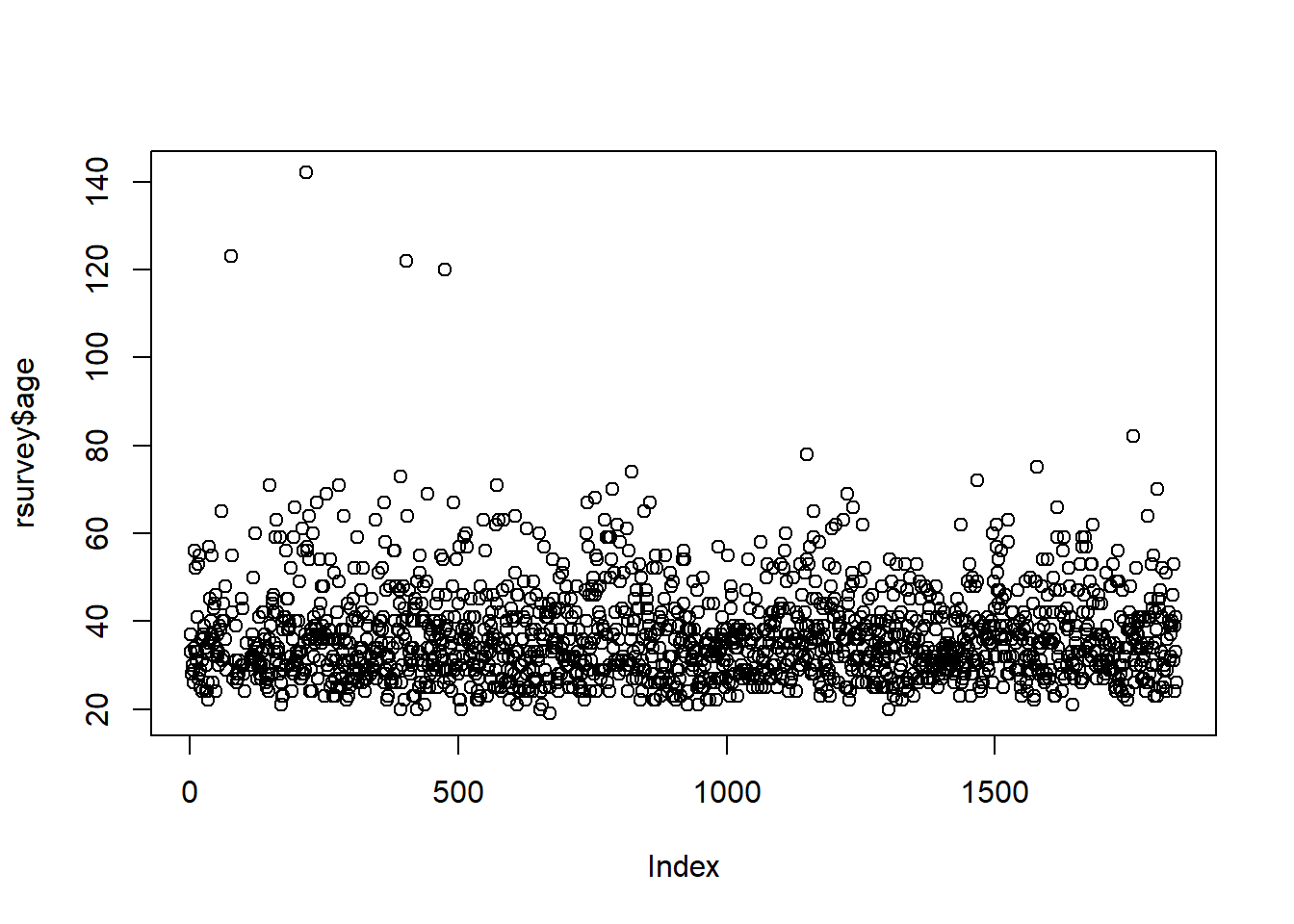
We can use a simple scatterplot for numerical data.
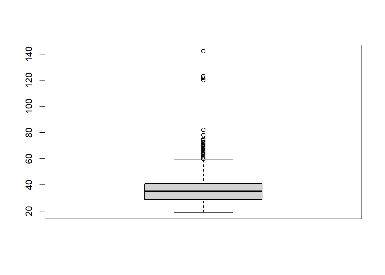
We could also use a boxplot:
Note: for more information on graphing data, see the Data Visualization chapters.
The graphs above shows that there are four possible outliers. These outliers have ages over 100. We can search for them in the data to see what is going on with them:
##   age qyear_born
## 1 123       1897
## 2 142       1878
## 3 122       1898
## 4 120       1900
It’s more than likely these are not serious responses, so we would need to deal with them in some way (see Dealing with Outliers).
2.16.1.1 Detecting Categorical Outliers
We can also see if a category contains any numeric outliers based on another variable. For example, if we want to see if there are any age outliers for the experience variable, we can use a simple boxplot:
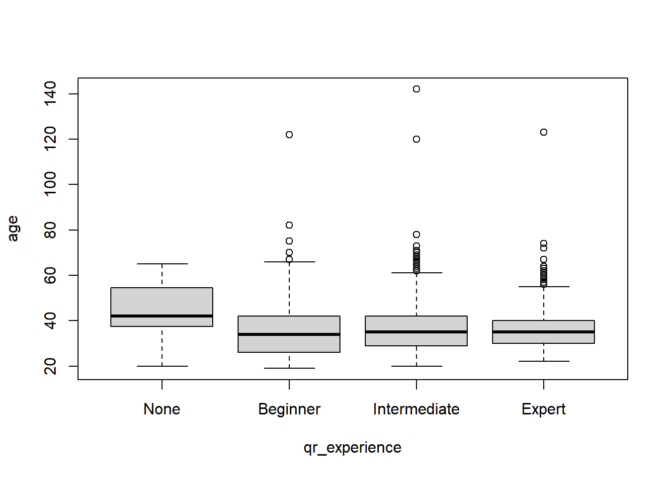
The graph above shows the four same extreme outliers. It also shows beginner, intermediate, and expert responses have some higher ages, but they don’t suggest any surprising outliers, especially because each of the three have high ages.
What does the code mean?
plot(- make a plotage ~ qr_experience,- plot age by (~) experiencedata=rsurvey)- from the “rsurvey” data frame
2.16.2 Detecting outliers with Z-scores
One way to detect outliers is to standardize values and select values greater than or less than some specific value. For example, Tabachnick and Fidell (2013) suggest any score above 3.29 may be an outlier for continuous, univariate data.
There are many ways to create Z-scores in R. You could do it manually:
rsurvey$z_of_age <- (rsurvey$age - mean(rsurvey$age, na.rm=T))/sd(rsurvey$age, na.rm = T)

# to check
summary(rsurvey$z_of_age)
## Min. 1st Qu. Median Mean 3rd Qu. Max. NA's
## -1.6178 -0.6992 -0.1480 0.0000 0.4032 9.6809 107However, we could also load a package and use a function to do it quickly. For example, the effectsize package has a standardize() function.
# install package if needed
# install.packages("effectsize")

rsurvey$z_of_age <- effectsize::standardize(rsurvey$age)

# to check
summary(rsurvey$z_of_age)
## Min. 1st Qu. Median Mean 3rd Qu. Max. NA's
## -1.6178 -0.6992 -0.1480 0.0000 0.4032 9.6809 1072.16.3 Dealing with Outliers
2.16.3.1 Removal
One thing you can do is “delete” your outliers. We will set outliers to NA.
# set ages over 100 to NA
rsurvey <- rsurvey %>%
  mutate(age2 = ifelse(age > 99, NA, age))

# check if we made the correct change
rsurvey %>%
  filter(qyear_born < 1901) %>%
  select(age2, qyear_born)
## age2 qyear_born
## 1 NA 1897
## 2 NA 1878
## 3 NA 1898
## 4 NA 1900Let’s look at the plot again:
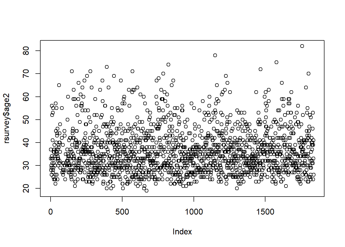
There are now no clear outliers for the “age” variable.
2.16.3.2 Filtering
Rather than deleting that data, you could simply use filter() to temporarily remove it. For example:

In the formula above, with() is a base R function that uses the data from a tidyverse chain (functions with %>%). Using strictly base R would require more steps, including creating a new data frame:

A Note about “Deleting” Values
It is never a good idea to delete or overwrite your raw data. Recall that we have a “raw_data” data object that we have not transformed in any way. All transformations have been done in new data objects and, sometimes, in new variables. This is good practice so that we can assess our changes and revert our changes if necessary.
2.16.3.3 Winsorizing
Winsorizing is a way to replace the most extreme scores with another value. The psych package has a winsor() function that will replace the top and bottom values with the next highest score.
For example, the code below trims the top and bottom 2% of the data set and replaces it with the next highest and lowest values.
library(psych)

winsored <- rsurvey %>%
  mutate(winsor = winsor(age, trim=.02, na.rm=T))

# let's check
winsored %>%
  select(age, winsor) %>%
  filter(age < 20 | age > 70)
## age winsor
## 1 123 63.4
## 2 71 63.4
## 3 142 63.4
## 4 71 63.4
## 5 73 63.4
## 6 122 63.4
## 7 120 63.4
## 8 71 63.4
## 9 19 22.0
## 10 74 63.4
## 11 78 63.4
## 12 72 63.4
## 13 75 63.4
## 14 82 63.42.17 Assessing Normality
2.17.1 Histograms
Normality can be visually assessed with a histogram. A quick histogram can be made using base R’s hist() function:
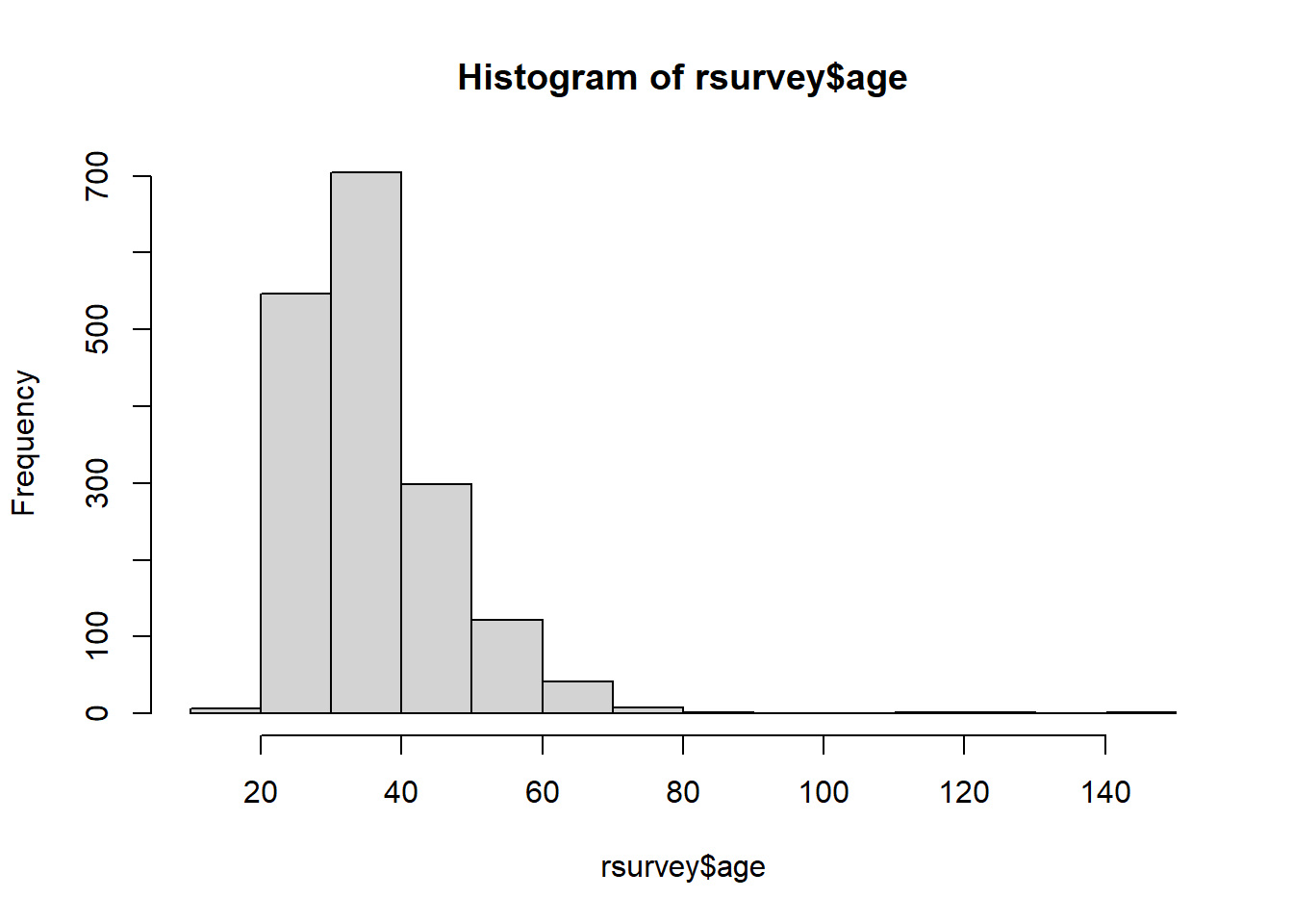
For additional information on creating more detailed and advanced histograms, See Data Visualization with ggplot
2.17.2 Density (Curve) Plots
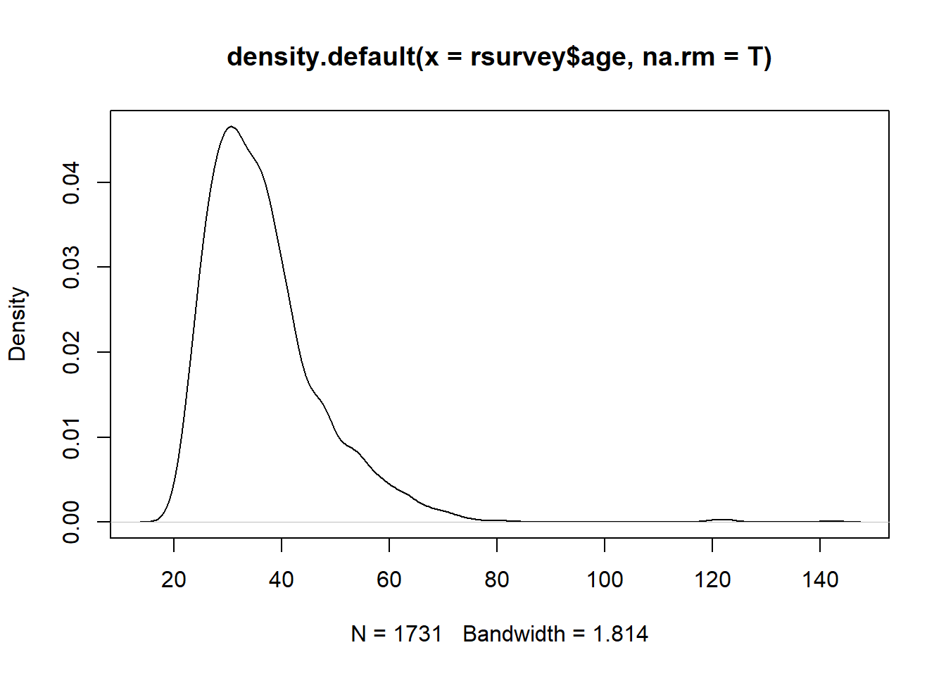
You can also use a density plot to visually assess normality:
2.17.4 Skewness and Kurtosis
There are a number of ways to get values for skewness and kurtosis.
You can get the values alongside other stats with the psych package’s describe()
You can also use skewness() and kurtosis() functions from the moments package:
## [1] 2.139836## [1] 11.492442.17.5 Tests of Normality
Univariate tests of normality are also easily done in R. The stats package (included with R) contains both the Kolmogorov-Smirnov (K-S) test and the Shapiro-Wilk’s test. The Shapiro-Wilk’s test is more common and easier to compute in R:
##
##  Shapiro-Wilk normality test
##
## data:  rsurvey$age
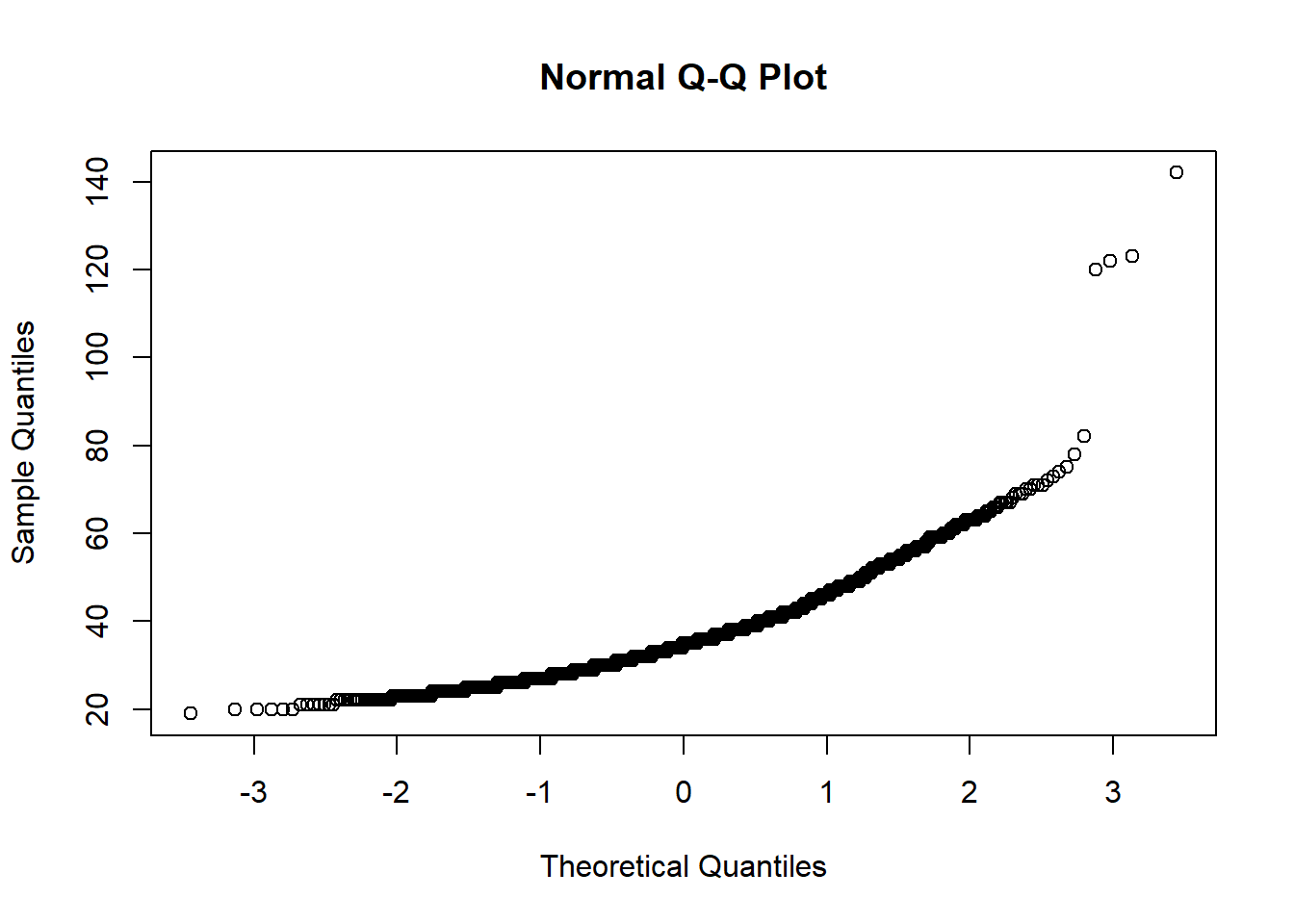
## W = 0.86577, p-value < 2.2e-16
The above p-value is significant at less than 0.05, signifying non-normality.
See ?shapio.test and ?ks.test for more information.
2.17.6 Transforming Variables
The following as some of the many methods you can use if you wish to deal with non-normality by transforming variables (DataNovia, n.d.):
- Square Roots
sqrt(x)for positive skewsqrt(max(x+1)-x)for negative skew
- Log
log10(x)for positive skewlog10(max(x+1)-x)for negative skew
- Inverse
1/xfor positive skew1/max(x+1)for negative skew
2.18 Identifying missing data
There are a number of ways to identify missing data in R.
2.18.1 Per Variable
We have already seen a number of ways to view and summarize data Viewing Your Data. There are several other functions that can be useful.
You can use is.na to get the proportion of NA values:
## [1] 0.05821545This means that around 6% of the “age” variable is missing.
Conversely, you can also use complete.cases to see how many cases are not missing:
## [1] 0.941784594% of the age variable is not missing.
2.18.2 Entire Data Frame
We can look at an entire data frame by using summarize_all, part of the summarize family of functions in dplyr (part of tidyverse).
This will produce a new data object where each column has 1 row, and that row is the percent missing.
What does the code mean?
missing <-- assign everything to a new data frame (this step is optional and you could just explore everything in the console)rsurvey %>%- use “rsurvey” andsummarize_all(- summarize every columnfuns(- use the following function (“funs”) to summarize everythingmean(is.na(.))))- take the mean of missing data.
- the
.in parentheses means to use the entire data frame- We need to include it because
is.narequires an argument
A Note on
summarize
summarizeis a family of verbs indplyrthat includessummarize,summarize_if,summarize_at(for specific columns), andsummarize_all. You may also see it spelled assummarise- this is the same function. Check out?summarize_allfor more information.
Let’s quickly view what this new missing object looks like using glimpse(). This will print the columns and first row vertically in the console. Because there are 67 columns, we will just look at the first 10.
## Rows: 1
## Columns: 10
## $ qtime                  <dbl> 0
## $ qr_experience          <dbl> 0.01686616
## $ qr_difficulty          <dbl> 0.9956474
## $ qr_length_to_success   <dbl> 0
## $ qhow_to_learn_r        <dbl> 0
## $ qreason_to_learn       <dbl> 0
## $ qr_use                 <dbl> 0
## $ qtools                 <dbl> 0
## $ qobstacles_to_starting <dbl> 0
## $ qr_year                <dbl> 0.08813928
You can also get a quick visual by running this code:
missing %>%
  pivot_longer(qtime:age2, names_to = "variable",
               values_to = "pct") %>%
  filter(pct > 0) %>%
  filter(!str_detect(variable, "use_")) %>%
  ggplot(aes(x=reorder(variable, pct), y=pct)) +
  coord_flip() +
  geom_col()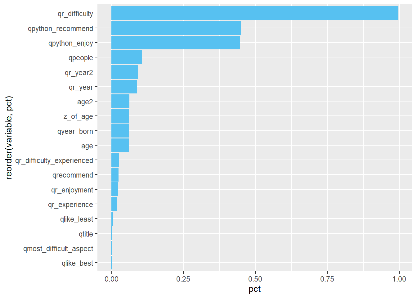
This code introduces some new concepts that will be covered later, so the following explanation will not go into detail.
What does the code mean?
missing %>%- use the “missing” data framepivot_longer(qtime:age2, names_to = "variable", values_to = "pct") %>%- our “missing” data frame had 1 row and 67 columns. By usingpivot_longer, we “flipped” our data frame so it had 2 columns (“variable” and “pct”) and 67 rows. This is easier to visualize.filter(pct > 0) %>%- we removed any columns with no missing datafilter(!str_detect(variable, "use_")) %>%we removed any columns that started with “use_” because those are check-all questions.
- note the
!at the beginning means “is not” or “does not”, so this says to filter any columns that does not start with “use_to”ggplot(aes(x=reorder(variable, pct), y=pct)) +- this line introduces a powerful visualization tool,ggplot, which will be covered later. It says to use “variable on the x-axis (and order it by”pct" so that it is in descending order) and use “pct” on the y-axis.
- Note that a quirk of
ggplotis that it uses+instead of%>%despite being part of thetidyversecoord_flip() +this will flip the visual to make the bar chart horizontalgeom_col()- this means we will make a column (bar) chart
See Data Visualization with ggplot for more information.
2.19 Dropping missing data
You can remove missing data by using drop_na().
If you use drop_na() without including columns in the (), it will drop rows that are missing values in any column. This will severely reduce your data frame. If we run the following code, it will drop everything and you will have 0 observations because every row has at least 1 missing value somewhere.
## [1] qtime                qr_experience
## [3] qr_difficulty        qr_length_to_success
## [5] qhow_to_learn_r
## <0 rows> (or 0-length row.names)
This command is useful if you have selected (with select() or subset()) a single column or a small group of columns and you do want to drop any missing data, but in general, you may want to specify columns:
This will remove all rows with missing data in the age variable. Compared “rsurvey” to “missing_dropped_some” and you will see less observations.
2.20 Replacing missing data with 0s
Sometimes missing data is meaningful and it would be useful in including them in various analyses. NA values are typically dropped from analyses, but we can include them by changing them to 0s. To do so, we can use mutate():
Let’s compare the mean age of our new data frame and our old one:
## [1] 36.61121## [1] 34.479872.21 Mean imputation
If warranted, we can easily replace missing data with means (or medians) like so:
mean_imputation <- rsurvey %>%
  mutate(age = ifelse(is.na(age), mean(age, na.rm=T), age))

mean(mean_imputation$age)
## [1] 36.611212.22 Multiple imputation
Multiple imputation is currently beyond the scope of this guide. However, you can learn more at any of the following sites:
