Chapter 4 Use case 3: `jointModel()` with multiple traditional gear types

This third use case will show how to fit and interpret the joint model with paired eDNA and traditional survey data when multiple traditional gear types have been used. These different gear types may have different expected catch rates, \(\mu\), represented by gear-specific catchability coefficients q.

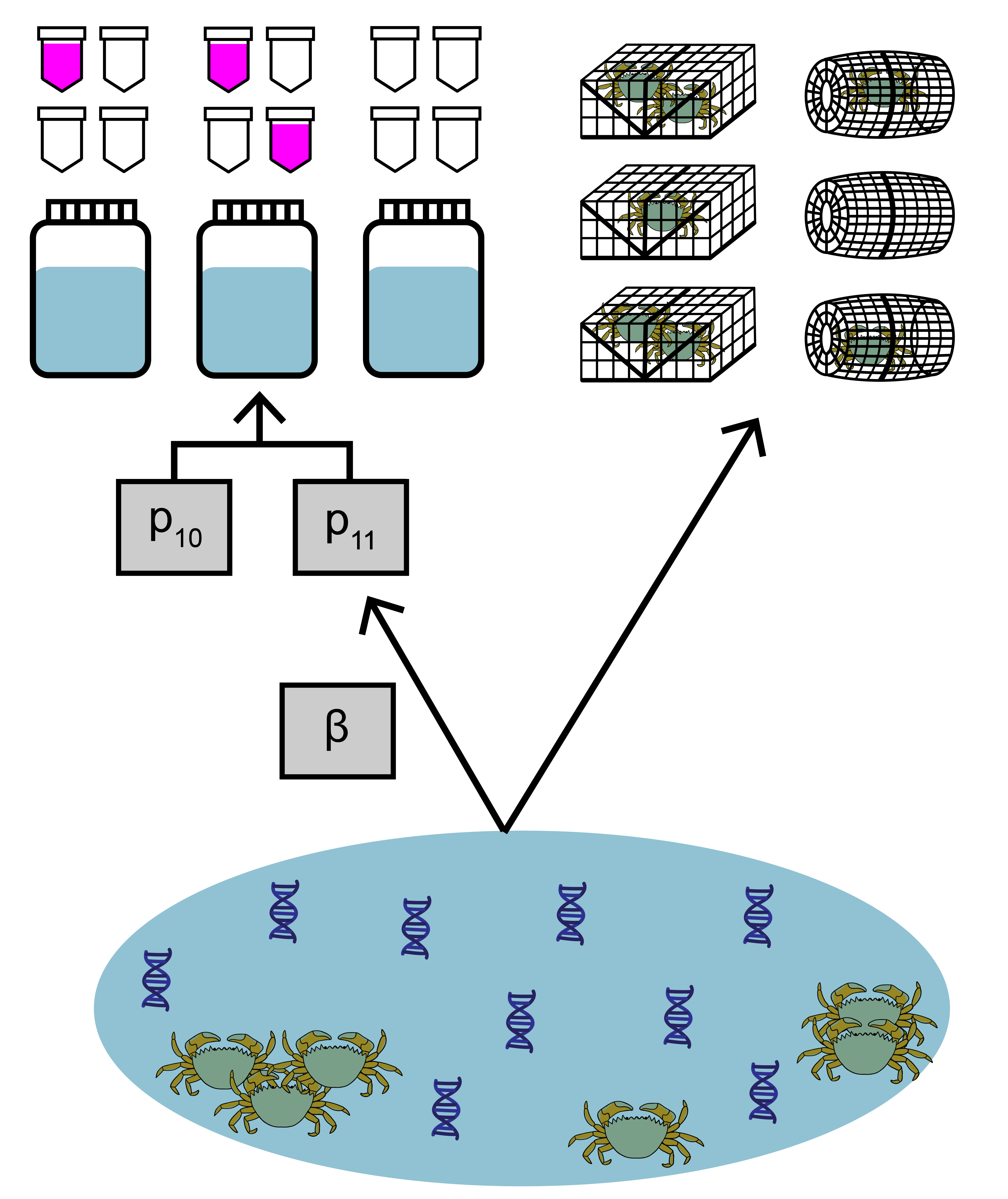
The data used in this example comes from a study by Keller et al. (2022) about invasive European green crab (Carcinus maenas) in Washington state. Environmental DNA samples were collected at 20 sites, along with paired baited trap sampling. The eDNA data is detection/non-detection data generated through quantitative polymerase chain reaction (qPCR).

4.1 Prepare the data

Similar to the goby data, the green crab data is still a list of matrices. Now, instead of data on site-level covariates, site.cov, there is data representing the gear type for each of the traditional samples, count.type.

library(eDNAjoint)
data(greencrabData)
names(greencrabData)

## [1] "qPCR.N"     "qPCR.K"     "count"      "count.type"

Again, all matrices should have the same number of rows (n=20), and rows across all four matrices should correspond to the same sites.

Let’s look at the count. This data is from baited trap sampling for green crab. Each integer refers to the catch of each trap (i.e., catch per unit effort, when effort = 1). The rows correspond to sites, and the columns refer to the replicated trap samples (secondary sample units) at each site, with a maximum of 420 samples.

dim(greencrabData$count)

## [1]  20 420

Blank spaces are filled with NA at sites where fewer trap samples were collected than the maximum. In this example, the count data are integers, but continuous values can be used in the model (see Eq. 1.3 in the model description).

greencrabData$count[1:6,1:20]

##      1 2 3 4 5 6  7  8  9 10 11 12 13 14 15 16 17 18 19 20
## [1,] 0 0 0 0 0 0  0  0  0  0  0  0  0  0  0  0  0  0  0  0
## [2,] 0 0 0 0 0 0  0  0  0  0  0  0  0  0  0  0  0  0  0  0
## [3,] 0 0 0 0 0 0  0  0  0  0  0  0  0  0  0  0  0  0  0  0
## [4,] 1 0 1 2 0 0  0  0  0  0  0  0  0  0  0  2  0  0  0  1
## [5,] 0 0 0 0 0 0  0  0 NA NA NA NA NA NA NA NA NA NA NA NA
## [6,] 0 0 0 0 0 0 NA NA NA NA NA NA NA NA NA NA NA NA NA NA

Next, let’s look at count.type, which consists of integer indicators of gear type for each trap sample. Here, 1 refers to the Fukui gear type, and 2 refers to the Minnow gear type.

greencrabData$count.type[1:6,1:20]

##      1 2 3 4 5 6  7  8  9 10 11 12 13 14 15 16 17 18 19 20
## [1,] 1 1 1 1 2 1  2  2  2  2  2  2  1  1  1  1  2  1  1  2
## [2,] 2 2 2 2 2 2  2  2  2  1  1  1  1  1  1  1  2  2  2  2
## [3,] 1 1 1 2 1 2  1  1  1  2  1  2  2  1  2  2  1  2  1  2
## [4,] 2 2 2 2 2 2  2  2  1  2  2  2  2  2  2  2  2  2  2  2
## [5,] 1 2 1 2 1 2  1  2 NA NA NA NA NA NA NA NA NA NA NA NA
## [6,] 2 1 2 1 2 1 NA NA NA NA NA NA NA NA NA NA NA NA NA NA

Note that the locations of the NAs in this matrix match count.

For more data formatting guidance, see section 2.1.1.

4.2 Fit the model

Now that we understand our data, let’s fit the joint model. The key arguments of this function include:

data: list of qPCR.K, qPCR.N, count, and count.type matrices
cov: no site-level covariates are included in this model
family: probability distribution used to model the trap count data. A negative binomial distribution is chosen here.
p10priors: Beta distribution parameters for the prior on the probability of false positive eDNA detection, \(p_{10}\). c(1,20) is the default specification.
q: logical value indicating the presence of multiple traditional gear types.

More parameters exist to further customize the MCMC sampling, but we’ll stick with the defaults.

# run the joint model with catchability coefficients
greencrab.fit.q.negbin <- jointModel(data = greencrabData, cov=NULL, family = 'negbin', 
                                     p10priors = c(1,20), q=TRUE)

4.3 Model selection

We previously made a choice to model the green crab count data with a negative binomial distribution. Perhaps we want to test how that model specification compares to a model specification where count data is modeled with a poisson distribution.

# run the joint model with poisson distribution
greencrab.fit.q.pois <- jointModel(data = greencrabData, cov=NULL, family = 'poisson', 
                                   p10priors = c(1,20), q=TRUE)

Let’s also fit some models where we assume that both gear types have the same catchability. We set q=FALSE to not estimate catchability coefficients.

# run the joint model with four covariates
greencrab.fit.negbin <- jointModel(data = greencrabData, cov=NULL, family = 'negbin', 
                                   p10priors = c(1,20), q=FALSE)
greencrab.fit.pois <- jointModel(data = greencrabData, cov=NULL, family = 'poisson', 
                                 p10priors = c(1,20), q=FALSE)

Now let’s perform model selection using leave-one-out cross validation.

# perform model selection
jointSelect(modelfits = list(
  # include catchability coefficient, model count data with negative binomial
  greencrab.fit.q.negbin$model, 
  # include catchability coefficient, model count data with poisson
  greencrab.fit.q.pois$model, 
  # include catchability coefficient, model count data with negative binomial
  greencrab.fit.negbin$model, 
  # include catchability coefficient, model count data with poisson
  greencrab.fit.pois$model))

##        elpd_diff se_diff
## model3    0.0       0.0 
## model1   -1.3       1.9 
## model4 -165.9      38.3 
## model2 -168.6      37.7

These results tell us that models one and three (models with and without catchability coefficients for the gear types) that use a negative binomial distribution for count data have similar Bayesian LOO estimates of the expected log pointwise predictive density (elpd_loo). Notably, a negative binomial distribution represents the data-generating process for our count data much better than a poisson distribution.

4.4 Interpret the output

4.4.1 Summarize posterior distributions

For the sake of illustration, let’s interpret the results of the model fit with catchability coefficients. Use jointSummarize() to see the posterior summaries of the model parameters.

jointSummarize(greencrab.fit.q.negbin$model, par = c('p10','beta','q'))

##       mean se_mean    sd  2.5% 97.5%    n_eff  Rhat
## p10  0.018   0.000 0.009 0.005 0.041 9861.725 1.001
## beta 1.264   0.003 0.252 0.779 1.758 8166.353 1.000
## q[1] 0.791   0.001 0.102 0.607 1.011 7052.649 1.000

This summarizes the mean, sd, and quantiles of the posterior estimates of \(p_{10}\), \(\beta\), and q, as well as the effective sample size (n_eff) and Rhat for the parameters.

The mean estimated probability of a false positive eDNA detection is ~0.01. beta is the parameter that scales the sensitivity of eDNA sampling relative to trap sampling. q[1] represents the catchability coefficient of gear type 2, which scales the catch rate of gear type 2 relative to gear type 1.

Now let’s look at the summary of mu.

jointSummarize(greencrab.fit.q.negbin$model, par = 'mu')

##           mean se_mean    sd  2.5%  97.5%     n_eff  Rhat
## mu[1,1]  0.106   0.000 0.027 0.060  0.167 11087.290 1.000
## mu[1,2]  0.084   0.000 0.023 0.046  0.134 12272.442 1.000
## mu[2,1]  0.033   0.000 0.034 0.001  0.124 12644.744 1.000
## mu[2,2]  0.026   0.000 0.027 0.001  0.098 12849.768 1.000
## mu[3,1]  0.017   0.000 0.018 0.000  0.065 11728.908 1.000
## mu[3,2]  0.013   0.000 0.014 0.000  0.051 11652.654 1.000
## mu[4,1]  0.679   0.001 0.109 0.486  0.913 10358.057 1.000
## mu[4,2]  0.534   0.001 0.091 0.376  0.727 13733.108 1.000
## mu[5,1]  0.101   0.001 0.112 0.002  0.391 12400.060 1.001
## mu[5,2]  0.079   0.001 0.087 0.002  0.308 12624.261 1.001
## mu[6,1]  0.118   0.001 0.131 0.002  0.474 12415.280 1.000
## mu[6,2]  0.093   0.001 0.103 0.002  0.362 12436.800 1.000
## mu[7,1]  0.013   0.000 0.013 0.000  0.046 11536.502 1.000
## mu[7,2]  0.010   0.000 0.010 0.000  0.036 11613.839 1.000
## mu[8,1]  0.305   0.003 0.287 0.013  1.057 12176.236 1.000
## mu[8,2]  0.240   0.002 0.228 0.010  0.812 12229.052 1.000
## mu[9,1]  0.033   0.000 0.032 0.001  0.121 12239.622 1.000
## mu[9,2]  0.026   0.000 0.025 0.001  0.094 12393.706 1.000
## mu[10,1] 1.053   0.003 0.247 0.654  1.608  9396.637 1.000
## mu[10,2] 0.826   0.002 0.191 0.513  1.257 12189.442 1.000
## mu[11,1] 0.302   0.003 0.283 0.010  1.066 11949.258 1.000
## mu[11,2] 0.238   0.002 0.224 0.008  0.836 11974.793 1.000
## mu[12,1] 0.022   0.000 0.022 0.000  0.082 11913.553 1.000
## mu[12,2] 0.017   0.000 0.017 0.000  0.065 11903.361 1.000
## mu[13,1] 7.695   0.014 1.314 5.510 10.658  8773.256 1.000
## mu[13,2] 6.028   0.008 0.986 4.412  8.185 13787.661 1.000
## mu[14,1] 0.119   0.000 0.020 0.083  0.163 10516.170 1.000
## mu[14,2] 0.093   0.000 0.016 0.065  0.127 12832.735 1.000
## mu[15,1] 0.767   0.005 0.535 0.121  2.162 11736.703 1.000
## mu[15,2] 0.603   0.004 0.425 0.096  1.709 11838.228 1.000
## mu[16,1] 3.817   0.007 0.654 2.691  5.245  8104.350 1.000
## mu[16,2] 2.986   0.004 0.462 2.182  3.998 12464.335 1.000
## mu[17,1] 0.162   0.002 0.179 0.004  0.655 11807.769 1.000
## mu[17,2] 0.128   0.001 0.144 0.003  0.514 12043.245 1.000
## mu[18,1] 3.323   0.012 1.110 1.745  6.037  9084.432 1.000
## mu[18,2] 2.609   0.009 0.882 1.346  4.739 10312.524 1.000
## mu[19,1] 3.953   0.008 0.728 2.764  5.592  8667.387 1.000
## mu[19,2] 3.102   0.005 0.578 2.148  4.382 11254.870 1.000
## mu[20,1] 0.119   0.001 0.070 0.025  0.290 13147.869 1.000
## mu[20,2] 0.093   0.000 0.055 0.020  0.232 13401.767 1.000

mu[1,1] corresponds to the expected catch rate at site 1 with gear type 1. mu[1,2] corresponds to the expected catch rate at site 1 with gear type 2. mu[2,1] corresponds to the expected catch rate at site 2 with gear type 1.

We can also use functions from the bayesplot package to examine the posterior distributions and chain convergence.

First let’s look at the posterior distribution for \(p_{10}\).

library(bayesplot)

# plot posterior distribution, highlighting median and 80% credibility interval
mcmc_areas(as.matrix(greencrab.fit.q.negbin$model), pars = 'p10', prob = 0.8)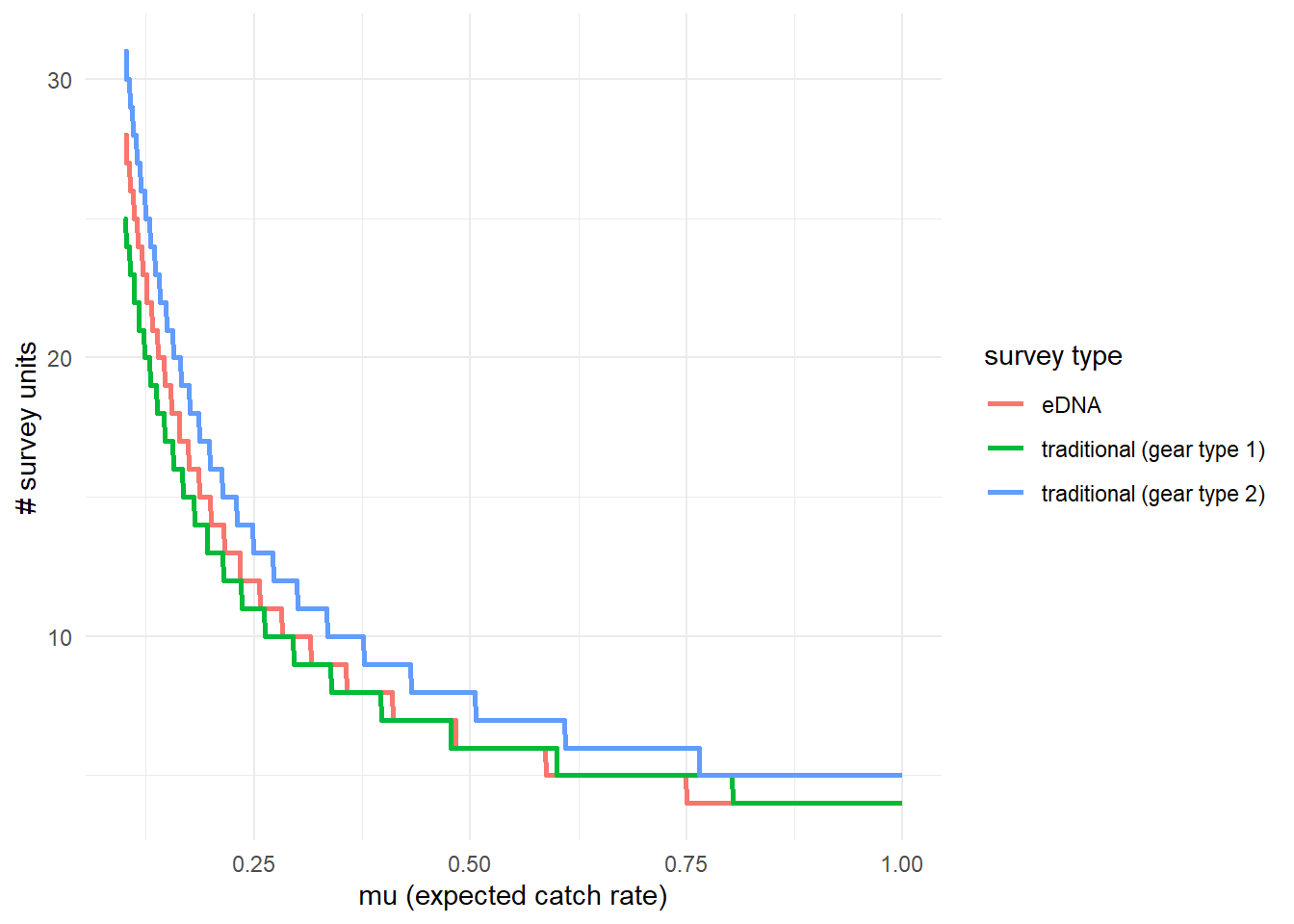

Next let’s look at chain convergence for \(p_{10}\) and \(\beta\).

# this will plot the MCMC chains for p10 and mu at site 1
mcmc_trace(rstan::extract(greencrab.fit.q.negbin$model, permuted = FALSE), 
           pars = c('p10', 'beta'))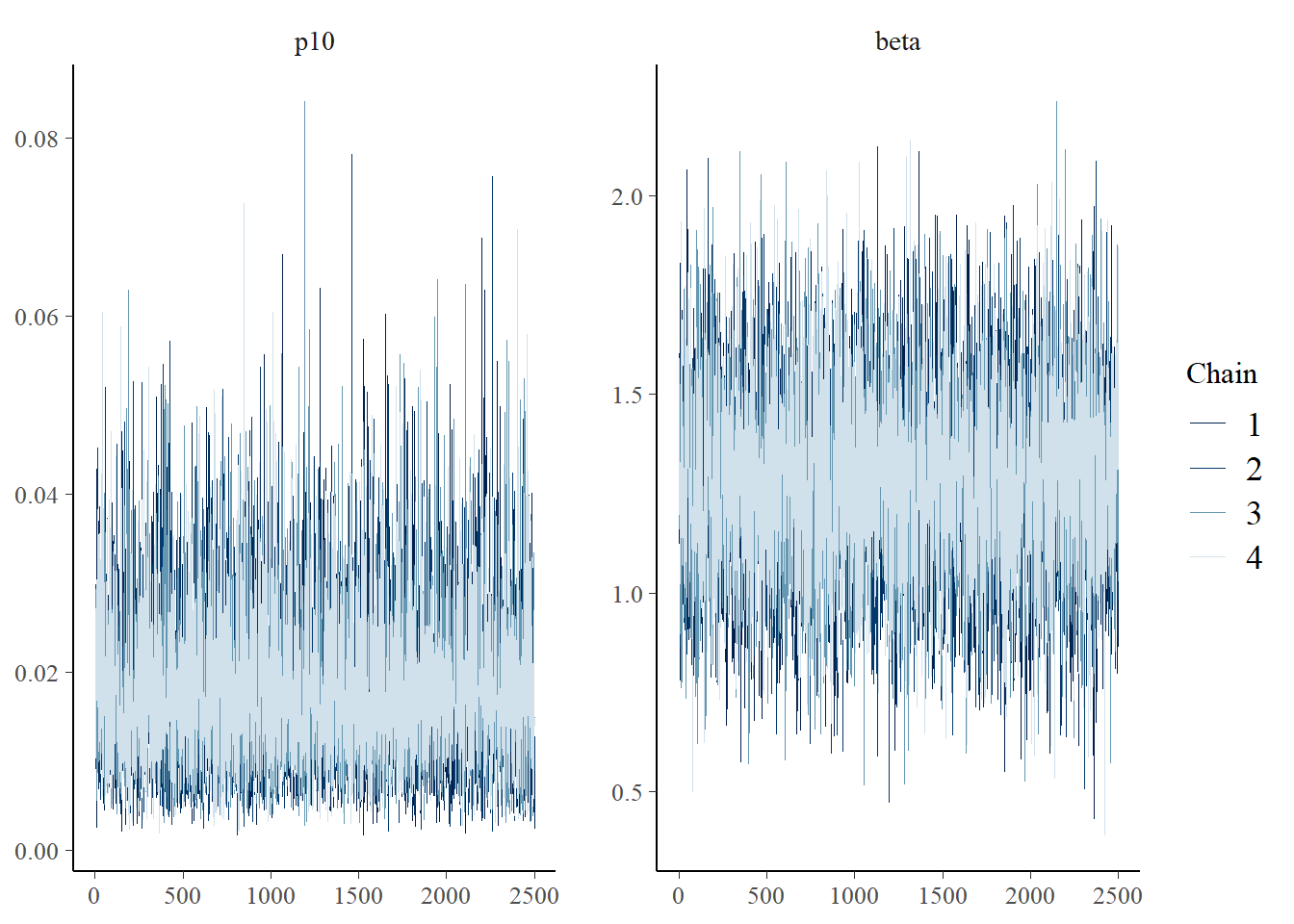

4.4.2 Effort necessary to detect presence

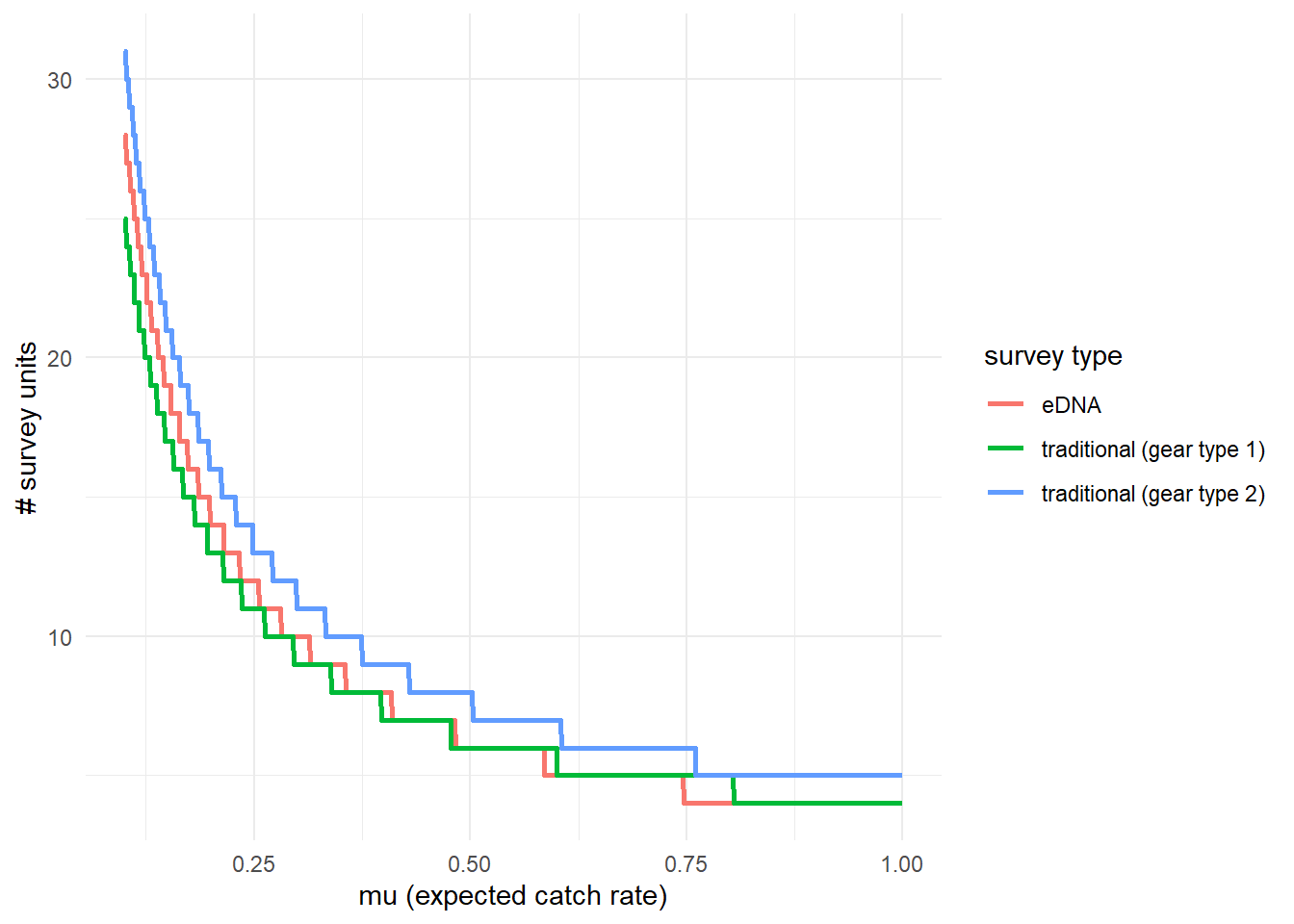
To further highlight these results, we can use detectionCalculate() to find the units of survey effort necessary to detect presence of the species. This function is finding the median number of survey units necessary to detect species presence if the expected catch rate, \(\mu\) is 0.1, 0.5, or 1. \(\mu\) now represents the expected catch rate of gear type 1.

detectionCalculate(greencrab.fit.q.negbin$model, mu = c(0.1,0.5,1), 
                   probability = 0.9)

##       mu n_traditional_1 n_traditional_2 n_eDNA
## [1,] 0.1              25              31     28
## [2,] 0.5               6               8      6
## [3,] 1.0               4               5      4

We can see that it takes 27 eDNA samples, 25 trap samples (gear type 1), and 31 trap samples (gear type 2) to detect green crab presence with 0.9 probability if the expected catch rate with gear type 1 is 0.1.

We can also plot these comparisons. mu.min and mu.max define the x-axis in the plot and represent the expected catch rate of gear type 1.

detectionPlot(greencrab.fit.q.negbin$model, mu.min = 0.1, 
              mu.max = 1, probability = 0.9)

4.4.3 Calculate \(\mu_{critical}\)

Now let’s calculate \(\mu_{critical}\), which is the value of \(\mu\) where the probability of a false positive eDNA detection equals the probability of a true positive eDNA detection.

muCritical(greencrab.fit.q.negbin$model, cov.val = NULL, ci = 0.9)

##               gear_1      gear_2
## median   0.060002140 0.047027009
## lower_ci 0.009341018 0.007563121
## upper_ci 0.133794971 0.105046465

This function calculates \(\mu_{critical}\) using the entire posterior distributions of parameters from the model, and ‘HDI’ corresponds to the 90% credibility interval calculated using the highest density interval. The first column corresponds to \(\mu_{critical}\) if gear type 1 is used, and the second columns corresponds to \(\mu_{critical}\) if gear type 2 is used.

4.5 traditionalModel()

In some circumstances, it may be helpful to model just the traditional survey data without eDNA data for comparison. Use traditionalModel here, which requires the following parameters:

data: list of count and (optionally) count.type matrices
family: probability distribution used to model the trap count data. A negative binomial distribution is chosen here.
q: logical value indicating the presence of multiple traditional gear types.