Chapter 1 Maths Background

Welcome to the Maths Background chapter. In this chapter, we will cover some maths symbols, meanings, and calculations which are fundamental to the statistical content in STM1001. Examples and practice exercises are included throughout this section for you to develop and test your knowledge.

For convenience, this chapter is divided into sections based on the different maths concepts covered. So, while one way to use this chapter is to read through it in its entirety, it is also designed so that you can focus on particular sections as needed.

1.1 Maths symbols and meanings

1.1.1 Absolute Value

The Absolute Value of a number is the size or magnitude of the number. We use the notation \(|x|\) to denote the absolute value of a some real number \(x\).

When reporting the absolute value, we simply ignore the original sign associated with the number: the absolute value will always be non-negative as we are considering the magnitude of the number. For example, \(|-5| = 5\), \(|2| = 2\), \(|-0.123| = 0.123\), etc.

1.1.2 Intervals

An interval of values refers to some number of sequential values within a certain range.

When reporting an interval of values, we denote the interval using the start and end points, separated by a comma.

For example, \([a, b]\) denotes the interval of values from \(a\) (the minimum) to \(b\) (the maximum) for some real numbers \(a\) and \(b\) where \(a \leq b\).

We can further refine our interval notation via our selection of brackets.

If we use round brackets - i.e. \((\) and \()\), these are non-inclusive. For \((a, b)\), the values \(a\) and \(b\) would not be included in the interval.
If we use square brackets - i.e. \([\) and \(]\), these are inclusive. For \([a, b]\), the values \(a\) and \(b\) would be included in the interval.
We can use a mixture of round and square brackets. For \([a, b)\) for example, the value \(a\) would be included in the interval but the value \(b\) would not be included in the interval. This interval would start at, and include, \(a\), and go all the way up to, but not include, \(b\).

1.1.3 Equality and inequality operators

If two mathematical terms are equivalent, we can use the notation \(=\) to denote that they are considered equal. For example if \(a=2\) and \(b=2\) we could write \(a=b\).

In many instances, two or more terms we are comparing or using in our calculations may not be equal. In such cases, we can use other notation to represent the relationships between these terms:

\(<\) is the less than sign - for example \(2 < 4\)
\(>\) is the greater than sign - for example \(5 > 1\)
\(\neq\) is the not equal sign - for example \(3 \neq 8\)

In some cases, we may be interested in values of at least or at most a certain amount. In such cases, we can use the notation:

\(\leq\) is the less than or equal to sign - for example \(a \leq 2\) for some real number \(a\) means that \(a\) is \(2\) or less.
\(\geq\) is the greater than or equal to sign - for example \(b \geq 4\) for some real number \(b\) means that \(b\) is \(4\) or more

If we have rounded any values we obtained in our calculation processes, we may like to note that our final results are not necessarily as precise as possible, by using the approximately equal to symbol \(\approx\) in place of \(=\).

For example, we know \(2 + 2 = 4\), but we could also say \(2.1 + 2.2 \approx 4\).

1.1.4 Division Symbols

A commonly used symbol for division is the \(\div\) symbol. Another symbol commonly used for division is the \(/\) symbol. For example, \(4\div 2\) is equivalent to \(4/2\). Fractions are also a form of division. For example, \(\displaystyle \frac{4}{2}\) is equivalent to both \(4\div 2\) and \(4/2\).

Division symbols

For two numbers \(a\) and \(b\), "\(a\) divided by \(b\)" can be expressed in any of the following equivalent ways:

\(a\div b\)
\(a/b\)
\(\displaystyle\frac{a}{b}\)

1.1.5 Scientific notation and E-notation

Sometimes we will deal with very large or very small numbers. These can become unwieldy to write in the normal way, and so for efficiency, we can instead write them in scientific notation format, aka E-notation or exponential notation.

In scientific notation, we re-express a value as a number times some power of 10.

Rule: Scientific Notation

The general format for numbers written in scientific notation is \[a \times 10^n \qquad \text{or equivalently } \qquad a\text{e}\pm n\]

where:

\(1 \leq a \leq 10\)
\(n\) is an integer (positive or negative)
e is shorthand for `times 10 to the power of'
- If n is positive, we would see \(a\text{e}+n\), while if n is negative, we would see \(a\text{e}-n\).

Example 1.1 Consider the value \(1.2 \times 10^5\). This is the scientific notation form of the number \(120000.\) To see this, we can:

Shift the decimal point in 1.2 five places to the right (adding zeroes as we pass 2) since 10 is raised to the power 5 here. Effectively, we are multiplying \(1.2\) by \(10^5 = 100000\).

Example 1.2 Consider the value \(4.5 \times 10^{-6}\). This is the scientific notation form of the number \(0.0000045.\) To see this, we can:

Shift the decimal point in 4.5 six places to the left (adding zeroes as we pass 4) since 10 is raised to the power of negative 6 here. Effectively, we are multiplying \(4.5\) by \(10^{-6} = 0.000001\), (or if you prefer, dividing \(4.5\) by \(10^6 = 1000000\)).

Example 1.3 Consider the value \(4.5E-6\). This is the exponential notation form of the number \(0.0000045\), so we can write this equivalently as \(4.5 \times 10^{-6}\).

Exercise 1.1 Solve the following problems:

Convert \(1.54 \times 10^{-4}\) to normal format
Convert \(3.17\text{e}-3\) to normal format
Convert \(8.293 \times 10^6\) to normal format

0.000154
0.00317
8293000

1.2 Maths calculations

1.2.1 Rounding and Decimal Places of Accuracy

We can use rounding to present data to a specified number of decimal places.

The number of decimal places of accuracy to which we round a number refers to the number of digits presented after the decimal point.

For example, the number \(5.12345\) has five decimal places of accuracy, whereas the number \(5.12\) has two decimal places of accuracy.

As you can see, the fewer the decimal places of accuracy, the less precise a rounded number will be. Even miniscule adjustments can have large impacts in practice (consider currency exchange rates or drug dosage amounts).

Rule: Rounding to a certain number of decimal places of accuracy

If you need to round a value to a certain number of decimal places \(d\), then the general process is:

Check the \(d+1^{th}\) number after the decimal point in your original number.
If this \(d+1^{th}\) number is 5 or more, we round up the \(d^{th}\) number one unit, otherwise we leave it as is
We then report the resultant value to the \(d\) decimal places of accuracy.

Example 1.4 Suppose we want to round the value 4.135 to \(d=2\) decimal places. We have:

Check the \(d+1 = 3\)rd value after the decimal point (5) and
Noting that \(5 \geq 5\), we round 4.135 up by adding one unit to the \(d^{th}\) number after the decimal point.
Our resultant value is 4.14, correct to 2 decimal places of accuracy.

Example 1.5 As a second example, suppose we want to round the value 4.133 to \(d=2\) decimal places. We have:

Check the 3rd value after the decimal point (3) and
Noting that \(3 < 5\), we do not add one unit to the \(d^{th}\) number after the decimal point, so that
Our resultant value is 4.13, correct to 2 decimal places of accuracy.

Note that it is strongly suggested that you work with exact values throughout your calculation process and only round your final results (if necessary), as otherwise you could encounter issues:

For example we know \(2.4 + 2.3 = 4.7 \approx 5\) but if you round 2.4 and 2.3 to the nearest whole number before adding them, we would obtain 4.

It is important to be careful about rounding values - imagine if you were being paid 2.4K and 2.3K for two separate jobs at an agency; would you prefer they rounded the values before or after adding them to determine your total pay?\(^{\star}\)

Exercise 1.2 Solve the following problems:

Round \(18.34581\) to 3 decimal places
Round \(-1.43\) to 1 decimal place
Round \(134.580\) to the nearest whole number

18.346
-1.4
135

\(^{\star}\) Of course, any rounding here would be in cents only one would hope.

1.2.2 Percentages and proportions

Consider the following table:

Table 1.1: Frequency table detailing number of Semester 2 STM1001 students at each campus (as at 24/08/24).
Location	Frequency
Albury-Wodonga	22
Bendigo	124
Bundoora	492
Online	274
Total	912

If we wanted to compare one campus to another, we could use percentages or proportions to do so.

A proportion is used to denote an amount of something relative to a whole amount. To obtain a proportion we simply divide our quantity of interest by the whole possible amount for that phenomenon.

Example 1.6 For example, suppose we are interested in STM1001 students at Bendigo. The amount of STM1001 students at Bendigo is 124 and the total or whole amount of students in STM1001 is 912. Therefore the proportion of STM1001 students who are enrolled at the Bendigo campus this semester is \[\dfrac{124}{912} \approx 0.136.\]

If we wanted to express this proportion as an amount or ratio out of 100, we could convert it to a percentage by multiplying it by 100. I.e. the proportion \(0.136\) is equivalent to the percentage \(0.136 \times 100 = 13.6\%\).

Similarly, we could write a percentage as a proportion by dividing it by 100.

Exercise 1.3 Solve the following problems:

What is the proportion of STM1001 students at the Albury-Wodonga campus, correct to 2 decimal places of accuracy?
What is the percentage of STM1001 students at the Bundoora campus, correct to 2 decimal places of accuracy?
If the percentage of STM1001 students at the Online campus is 30%, what is this as a proportion?

0.02
53.95
0.3

1.2.3 Squares, square roots and powers

Squares

The square of a number is the number times itself and is denoted with a \(^2\) after the number. For example, if we wish to square some number \(x\), we write it as \(x^2\), which is equal to \(x \times x\). The term \(x^2\) can be referred to as "\(x\) squared".

Example 1.7 In this example, we square the following numbers, (a) 4, (b) 35, (c) 5.8467, as follows:

\(4^2 = 4 \times 4 = 16\)
\(35^2 = 35 \times 35 = 1225\)
\(5.8467^2 = 5.8467 \times 5.8467 = 34.1839\)

Exercise 1.4 Solve the following problems:

\(5^2\)
\(79^2\)
\(3.5375^2\). Round your answer to four decimal places.

25
6241
12.5139

Square roots

The square root of a number is the opposite of a square: it is the number which, if multiplied by itself, gives the original number. For example, if \(a^2 = b\), then \(a\) is the square root of \(b\). Another way of putting it: if we are asked to find the square root of some number \(b\), we can ask, "what number times itself is equal to \(b\)?" Square roots are represented using the "\(\sqrt{}\)" symbol. For example, the square root of \(b\) can be written as \(\sqrt{b}\).

Example 1.8 In this example, we take the square root of the following numbers, (a) 4, (b) 35, (c) 5.8467, as follows:

\(\sqrt{4} = 2\)
\(\sqrt{35} = 5.91608\)
\(\sqrt{5.8467} = 2.417995\)

Exercise 1.5 Solve the following problems:

\(\sqrt{9}\)
\(\sqrt{83}\). Round your answer to four decimal places.
\(\sqrt{4.9651}\). Round your answer to four decimal places.

3
9.1104
2.2283

Exercise 1.6 (Application) Recall that:

The variance is the standard deviation squared
The standard deviation is the square root of the variance.

Using these facts, solve the following problems:

Suppose a sample standard deviation was calculated to be 9. Then what would be the associated variance?
Suppose a sample variance was calculated to be 121 Then what would be the associated standard deviation?
Suppose a sample standard deviation was calculated to be 6.85. Then what would be the associated variance?
Suppose a sample variance was calculated to be 75.62 Then what would be the associated standard deviation? Round your answer to three decimal places.

81
11
46.9225
8.696

Taking the square root of a squared number

If we take the square root of a square number, the square and the square root cancel each other out, so that we are left with the original number. For example, \(\sqrt{a^2}\) is simply equal to \(a\).

Rule: Taking the square root of a squared number

\[\sqrt{a^2} = a\]

Example 1.9 Suppose we wish to take the square root of \(8^2\). We have:

\[\begin{align} \sqrt{8^2} &= \sqrt{64} \\ &= 8. \end{align}\]

However, using the rule that \(\sqrt{a^2} = a\), we can simplify this process as: \[\sqrt{8^2} = 8\]

Exercise 1.7 Solve the following problems:

\(\sqrt{9^2}\)
\(\sqrt{83^2}\)
\(\sqrt{4.9651^2}\)

9
83
4.9651

Exercise 1.8 (Application) Since \(\sqrt{a^2} = a\), it is often convenient to express the variance as some number squared, so that the square root of that number, the standard deviation, is immediately obvious. Using the fact that \(\sqrt{a^2} = a\), answer the following questions.

Suppose that \(X \sim N(10, 3^2)\). What is the standard deviation of \(X\)?
Suppose that \(X \sim N(10, 11^2)\). What is the standard deviation of \(X\)?
Suppose that \(X \sim N(5, 2.93^2)\). What is the standard deviation of \(X\)?
Suppose that \(X \sim N(7, 5.2945^2)\). What is the standard deviation of \(X\)?

Remember that if \(X \sim N(a, b^2)\), then the variance of \(X\) is \(b^2\).

3
11
2.93
5.2945

Powers

Squares and square roots are both examples of 'powers'. A power is the small number to the right of a number or letter. For example, if we consider \(8^2\), the power is the \(^2\) to the right of the \(8\). The term \(8^2\) can be read as either, "\(8\) squared", or "\(8\) to the power of \(2\)".

Similarly, a square root is actually equivalent to the power of \(\frac{1}{2}\). For example, \(\sqrt{8} = 8^{\frac{1}{2}}\). In words, we could say that "the square root of \(8\)" is equivalent to "\(8\) to the power of \(\frac{1}{2}\)".

A related term, which will become useful in Section 1.2.5, is order, which is a general term that can refer to powers and roots.

1.2.5 Order of operations

When faced with a mathematical expression, it is important that we know which order to carry out the operations, or calculations, within the equation. If we carry these out in the incorrect order, this can easily lead to an incorrect answer. For example, consider the simple expression, \[5 + 6 \times 7.\]

If we carry out the operations from left to right, we have:

\[\begin{align} 5 + 6 \times 7 &= 11 \times 7 \\ &= 77. \end{align}\]

If we carry out the multiplication first, followed by addition, we have:

\[\begin{align} 5 + 6 \times 7 &= 5 + 42 \\ &= 47. \end{align}\]

Clearly, \(77\) and \(47\) are two very different answers depending on the approach. Thankfully, there is a standard approach within mathematics which specifies the order in which to carry out the operations within a mathematical equation. This order can be remembered using the acronym BODMAS:

Brackets
Order (powers and roots)
Division
Multiplication
Addition
Subtraction

Using this acronym helps us to remember the following order:

Brackets
Orders (powers and roots)
Division and Multiplication. These operations have equal rank, so operations are carried out from left to right as they appear in the equation.
Addition and Subtraction. These operations have equal rank, so operations are carried out from left to right as they appear in the equation.

We will now consider some examples.

Example 1.14 Evaluate \(5 + 6 \times (2+4) - 7\). We have:

\[\begin{align} 5 + 6 \times (2+4) - 7 &= 5 + 6 \times 6 - 7 \;\;\;\;\;\hfill\text{(carry out the operation inside the brackets first)}\\ &= 5 + 36 - 7 \;\;\;\;\;\hfill\text{(carry out multiplication before addition and subtraction)}\\ &= 41 - 7 \;\;\;\;\;\hfill\text{(left to right, since addition and subtraction have equal rank)}\\ &= 34 \;\;\;\;\;\hfill\text{(final answer)}\\ \end{align}\]

Example 1.15 Evaluate \(3 - 5^2 \times (10 - 6)\). We have:

\[\begin{align} 3 - 5^2 \times (10 - 6) &= 3 - 5^2 \times 4 \;\;\;\;\;\hfill\text{(brackets first)}\\ &= 3 - 25 \times 4 \;\;\;\;\;\hfill\text{(order next)}\\ &= 3 - 100 \;\;\;\;\;\hfill\text{(multiplication next)}\\ &= -97 \;\;\;\;\;\hfill\text{(final answer)}\\ \end{align}\]

Exercise 1.11 Solve the following problems:

Evaluate \(9 - 4 \times (6+4) + 7\).
Evaluate \(3^2 - 49 \div (16-9) - 2\).
Evaluate \((10^2 - 92)\times(15 - 9)\div 8 + 10\).
Evaluate \(52^2 - 642 - 8\times(12^2 - 150)\).

-24
0
16
2110

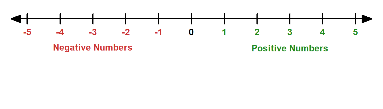
1.2.6 Negative numbers

Numbers can be positive, negative, or neither positive nor negative. Consider the number line shown below. Positive numbers are those numbers greater than zero, that is, \(> 0\). Negative numbers are those numbers less than zero, that is, \(< 0\). The number \(0\) is neither positive nor negative.

We can use the \(+\) sign in front of a number to indicate that it is positive: for example, \(+4\) is positive. We can use a \(-\) sign in front of a number to indicate that it is negative: for example, \(-4\) is negative. If there is no sign in front of a number, then we can assume it is positive, unless of course the number is \(0\).

Addition and Subtraction

Suppose we are either adding or subtracting positive numbers. Addition of positive numbers involves moving to the right on the number line. Subtraction of positive numbers involves moving to the left on the number line. However, this becomes more complicated when we are adding or subtracting negative numbers. Consider the following rules.

Rules for addition and subtraction of positive and negative numbers

Two positives \((+ \text{ and } +)\) remain a positive \((+)\)
Two negatives \((- \text{ and } -)\) become a positive \((+)\)
A positive and a negative \((- \text{ and } +\), in either order\()\) become a negative \((-)\)

Example 1.16 Evaluate \(5 + (-2) + 4 - 3 - (-5)\). We have:

\[\begin{align} 5 + (-2) + 4 - 3 - (-5) &= 5 -2 + 4 - 3 - (-5) \;\;\;\;\;\hfill [5 + (-2)\text{ becomes }5-2]\\ &= 5 -2 + 4 - 3 +5 \;\;\;\;\;\hfill [3 - (-5)\text{ becomes }3 + 5]\\ &= 9 \end{align}\]

Exercise 1.12 Solve the following problems:

Evaluate \(9 - (-2) - 4 - 3 + (-2)\).
Evaluate \(-11 - 4 - (-9) + (-7) + 3\).

Multiplication and Division

Consider the following rules, which we can use to determine the sign of the answer when multiplying or dividing positive and/or negative numbers.

Rules for multiplication and division of positive and negative numbers

A positive \(\text{ }\times \text{ or } \div\text{ }\) a positive will be positive \((+)\)
A positive \(\text{ }\times \text{ or } \div\text{ }\) a negative will be negative \((-)\)
A negative \(\text{ }\times \text{ or } \div\text{ }\) a positive will be negative \((-)\)
A negative \(\text{ }\times \text{ or } \div\text{ }\) a negative will be positive \((+)\)

Example 1.17 Consider the following examples.

\(7\times 3 = 21\)
\(7 \times (-3) = -21\)
\((-27)\div 3 = -9\)
\((-27)\div (-3) = 9\)
\(\displaystyle \frac{-3}{4} = -\frac{3}{4}\)
\(\displaystyle \frac{3}{-4} = -\frac{3}{4}\)
\(\displaystyle \frac{-3}{-4} = \frac{3}{4}\)

Exercise 1.13 Solve the following problems:

Evaluate \(7 \times (-6)\).
Evaluate \(-52 \times 64\).
Evaluate \(55 \div (-11)\).
Evaluate \(-824 \div (-63)\), and round your answer to four decimal places.

-42
-3328
-5
13.0794

1.2.7 Summation

In mathematics, the \(\sum\) sign is often used as a 'summation sign'. Using this sign allows us to write many equations in a simple and compact form. For example, consider the values \(x_1\) to \(x_5\) as follows:

\[ x_1 = 2; x_2 = 50; x_3 = 300; x_4 = 10; x_5 = 25.\]

Also suppose that we wish to add these five numbers together. We could express this sum as

\[\sum_{i = 1}^5 x_i,\] which is equal to \(x_1 + x_2 + x_3 + x_4 + x_5\). We also have that

\(i\) is called the 'index variable'. This is a general index that can that can take any of the values \(1, \ldots, 5\)
Underneath the summation sign, we have \(i = 1\). This tells us that we start by letting the index equal 1. That is, we start the summation with the value \(x_1\)
On top of the summation sign we have \(5\). This tells us the last index will be \(i = 5\). That is, the last element in the sum will be equal to \(x_5\)
The argument of the summation sign is \(x_i\)

Putting all of this together, we can read \(\displaystyle \sum_{i = 1}^5 x_i\) in words as, "The sum of \(x_i\) from \(i = 1\) to \(5\)".

Generalising this concept slightly, suppose we now have \(n\) values, or observations: \(x_1, x_2, \ldots, x_n\). Further suppose that we wish to add these \(n\) values together. We could express this sum as

\[\sum_{i = 1}^n x_i,\] which can be expressed in words as, "The sum of \(x_i\) from \(i = 1\) to \(n\)". This sum is equal to \(x_1 + x_2 + \ldots + x_n\).

Example 1.18 Consider the following observations:

\[ x_1 = 2; x_2 = 50; x_3 = 300; x_4 = 10; x_5 = 25.\]

Using these values, \(\displaystyle \sum_{i = 1}^5 x_i\) can be evaluated as

\[\begin{align} \sum_{i = 1}^5 x_i =& x_1 + x_2 + x_3 + x_4 + x_5 \\ =& 2 + 50 + 300 + 10 + 25 \\ =& 387. \end{align}\]

Exercise 1.14 Solve the following problems:

Using the values \(x_1 = 437; x_2 = 38; x_3 = 470; x_4 = 135,\) evaluate \(\displaystyle \sum_{i = 1}^4 x_i\).
Using the values \(x_1 = 90; x_2 = 276; x_3 = 220; x_4 = 115; x_5 = 179; x_6 = 457,\) evaluate \(\displaystyle \sum_{i = 1}^6 x_i\).

1080
1337

1.2.8 Calculating means

Note: the notation used in this section is included in Section 2.1.

The mean of a set of values, often referred to as the average, can be calculated by adding the set of values together, and then dividing that sum by the number of values. For example, suppose we wish to calculate the mean of the two values \(25\) and \(30\). We can calculate the mean as

\[(25 + 30)\div 2 = 55 \div 2 = 27.5.\]

This is a relatively simple rule to remember when we have a small number of values. However, it is useful to refer to a general formula for the mean that can apply to any number of values. Consider the following formula:

Formula for the sample mean

Suppose we have a sample of \(n\) numbers, and we wish to calculate the sample mean, which we denote \(\overline x\). The formula for the sample mean is:

\[\overline{x} = \dfrac{1}{n} \sum_{i=1}^{n} x_i\]

Example 1.19 Suppose we wish to calculate the mean of the following observations:

\[ x_1 = 2; x_2 = 50; x_3 = 300; x_4 = 10; x_5 = 25.\]

Using the formula for the sample mean, we can calculate the mean as

\[\begin{align} \overline{x} = &\frac{1}{n} \sum_{i = 1}^n x_i\\ =&\frac{1}{5}\sum_{i = 1}^5 x_i \\ =& \frac{1}{5}(x_1 + x_2 + x_3 + x_4 + x_5) \\ =& \frac{1}{5}(2 + 50 + 300 + 10 + 25) \\ =& \frac{1}{5}(387)\\ =& 77.4 \end{align}\]

Exercise 1.15 Use the formula for the sample mean to solve the following problems:

Calculate the mean of the values \[x_1 = 437; x_2 = 38; x_3 = 470; x_4 = 135.\]
\(\overline{x} =\)
Calculate the mean of the values, rounding your answer to four decimal places: \[x_1 = 90; x_2 = 276; x_3 = 220; x_4 = 115; x_5 = 179; x_6 = 457.\] \(\overline{x} =\)

270
222.8333

1.2.9 Calculating variance

Since we make use of the statistical software packages available to us, calculating the variance by hand is beyond the scope of what is required in STM1001. However for completeness, we provide the formula here, with an example and exercises for practice.

Formula for the sample variance

The formula for the sample variance, denoted by \(s^2\), is given as

\[s^2 = \frac{1}{n-1}\sum_{i=1}^{n}(x_i-\overline{x})^2\]

Example 1.20 Suppose we wish to calculate the variance of the following observations:

\[x_1 = 2; x_2 = 50; x_3 = 300; x_4 = 10; x_5 = 25.\]

From Example 1.19, we have that \(\overline{x} = 77.4\). Using this information, and the formula for the sample variance, we can calculate the variance as

\[\begin{align} s^2 =& \frac{1}{n-1}\sum_{i=1}^{n}(x_i-\overline{x})^2 \\ =& \frac{1}{5-1}\sum_{i=1}^{5}(x_i-77.4)^2 \\ =& \frac{1}{4}\left[(2-77.4)^2 + (50-77.4)^2 + (300-77.4)^2 + (10-77.4)^2 + (25-77.4)^2\right] \\ =& \frac{1}{4}\left[(-75.4)^2 + (-27.4)^2 + (222.6)^2 + (-67.4)^2 + (-52.4)^2\right] \\ =& \frac{1}{4}\left(5685.16+ 750.76 + 49550.76 + 4542.76 + 2745.76\right) \\ =& \frac{1}{4}(63275.2) \\ =& 15818.8 \end{align}\]

Of course, we can now calculate the sample standard deviation as

\[s = \sqrt{s^2} = \sqrt{15818.8} = 125.7728.\]

Exercise 1.16 Use the formula for the sample variance, as well as your answers to Exercise 1.15, to solve the following problems. Round your answers to four decimal places where relevant.

For the values \(x_1 = 437; x_2 = 38; x_3 = 470; x_4 = 135,\) calculate the following.
1. Sample variance:
2. Sample standard deviation:
For the values \(x_1 = 90; x_2 = 276; x_3 = 220; x_4 = 115; x_5 = 179; x_6 = 457,\) calculate the following.
1. Sample variance:
2. Sample standard deviation:

1. 46646
2. 215.9769
1. 17772.5667
2. 133.3138

1.2.10 Calculating \(z\)-scores

We can think of a \(z\)-score as a standardised value. The value of a \(z\)-score can tell us how far above or below the mean a value is. It can also be thought of as the number of standard deviations above or below the mean.

\(z\)-scores are discussed in more detail in Topic 3. Here, we focus on their calculation. Consider the following formula.

\(z\)-score formula

For a given observation \(x\) sampled from a distribution with mean \(\mu\) and standard deviation \(\sigma\), the \(z\)-score can be calculated as

\[z = \frac{x - \mu}{\sigma}\]

Example 1.21 Suppose university students' heights follow a \(N(172.38, 9.85^2)\) distribution. For a height of 182.23, we can calculate the \(z\)-score as follows.

First, we write down the information we know:

The observed height is \(x = 182.23\)
The mean is \(\mu = 172.38\)
The standard deviation is \(\sigma = 9.85\) (since the variance is \(\sigma^2 = 9.85^2\))

Using the \(z\)-score formula, we have

\[\begin{align} z =& \frac{x - \mu}{\sigma}\\ =& \frac{182.23 - 172.38}{9.85} \\ =& \frac{9.85}{9.85} \\ =& 1 \end{align}\]

Exercise 1.17 Use the \(z\)-score formula to solve the following problems. Round your answers to four decimal places where relevant.

For an observed value of 165 sampled from a \(N(172.38, 9.85^2)\) distribution, calculate the associated \(z\)-score:
For an observed value of -6 sampled from a \(N(-10, 4)\) distribution, calculate the associated \(z\)-score:
For an observed value of 28 sampled from a \(N(30, 4^2)\) distribution, calculate the associated \(z\)-score:

-0.7492
2
-0.5

1.3 Graphs

A graph is a visual representation of data. Visualising data is an intrinsic part of Statistics, and we can use graphs at various stages of our analyses to present, summarise and convey information. Graphs can focus on one or more variables of interest. The majority of the graphs we use in STM1001 are covered in the early weeks of content:

Bar charts, pie charts and histograms are discussed in the Topic 1 readings here
Scatter plots, box plots and violin plots are discussed in the Topic 2 readings here

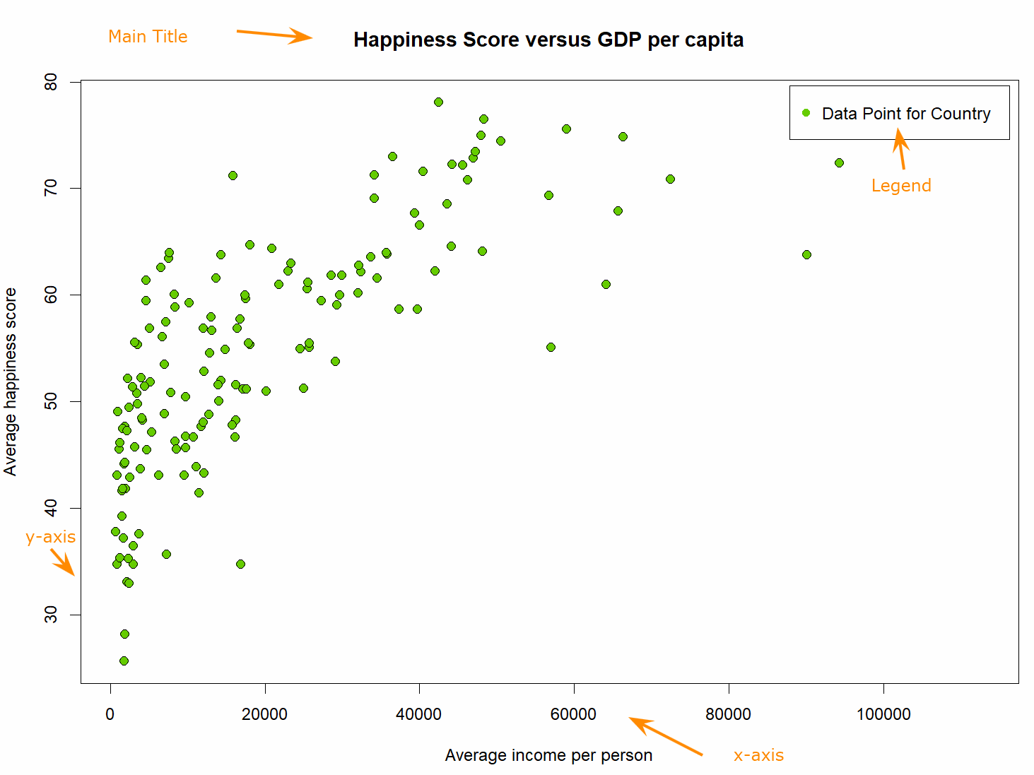
To clarify the information presented in a graph, we often include a legend to convey key details. The legend is typically seen in the top left or top right of a graph.

Scatter plots

If we are using a graph to plot data for two continuous numeric variables (i.e. if we are creating a scatter plot), there are several features to which we typically refer. These are outlined below:

Scatter plots are typically plotted using the Cartesian coordinate system in two dimensions. We have two perpendicular straight lines - the axes (pronounced `aks-ease', not like the weapon), which intersect at the point \((0, 0)\).

The horizontal axis is often called the \(x\)-axis. We typically plot our independent variable along the \(x\)-axis.
The vertical axis is often called the \(y\)-axis. We typically plot our dependent variable along the \(y\)-axis.

An example scatter plot is shown below, with key features noted using orange arrows.

STM1001: Maths and Notation Summary

Chapter 1 Maths Background

1.1 Maths symbols and meanings

1.1.1 Absolute Value

1.1.2 Intervals

1.1.3 Equality and inequality operators

1.1.4 Division Symbols

1.1.5 Scientific notation and E-notation

1.2 Maths calculations

1.2.1 Rounding and Decimal Places of Accuracy

1.2.2 Percentages and proportions

1.2.3 Squares, square roots and powers

1.2.4 Fractions, squares and square roots

1.2.5 Order of operations

1.2.6 Negative numbers

1.2.7 Summation

1.2.8 Calculating means

1.2.9 Calculating variance

1.2.10 Calculating \(z\)-scores

1.3 Graphs