STM1001 Topic 1: Introduction to statistics and presenting data
2023-09-27
Introduction to statistics
Where are we headed in this subject?
In this subject, we will be learning how to Make Sense of Data. One of the most important tools we can use to do so is Statistics.
What is Statistics?
Statistics allows us to make sense of data. It involves collecting, describing, and analysing data, and sometimes drawing conclusions from data.
In a nutshell, the above definition describes exactly what we will be doing throughout this subject. We will be learning about how to collect data. Once we have a data set, how can we then make sense of it? It is always a good idea to begin by describing the data. This helps to give us an overview of what the data may be telling us. Further analysis can help us to then draw conclusions about what we are seeing in the data: in other words, we may seek to make inferences about the data. Much of the time, we take a sample of data from a larger population, and use what we observe in the sample to make inferences about the population. In order to do this, we need to allow for some measure of uncertainty about the conclusions (inferences) we are drawing. Probability models allow us to do this.
Descriptive Statistics
Descriptive statistics involves summarising and displaying data via graphical and numerical means.
The table below displays the number of episodes in each season of popular television series, Breaking Bad (Wikipedia 2021). This is called a frequency table.
| Season | Season_1 | Season_2 | Season_3 | Season_4 | Season_5A | Season_5B |
| Number of Episodes | 7 | 13 | 13 | 13 | 8 | 8 |
Now suppose we were interested in looking at the average ratings during Seasons 1 to 3, and comparing them with the average ratings during Seasons 4 to 5B. Further suppose that we don't know what the ratings were for every episode, but we have the following observed ratings (in millions) for a random selection of five episodes from both groups:
\[1.73, 2.29, 1.89, 1.75, 1.67 \] We may now wish to summarise the above data to help us gain more insight about it. For example, consider the below table, which shows us the estimated average (or mean) number of US views per episode based on our sample:
| Seasons 1 to 3 | Seasons 4 to 5B | |
| Estimated Mean | 1.398 | 1.866 |
We can see that the estimated average views in Seasons 4 to 5B is higher than for Seasons 1 to 3. Another way to gain insight about our sample of data is to create a boxplot, such as the one pictured below:

By studying the boxplots, it becomes arguably even more obvious that Breaking Bad, on average, seems to have had higher ratings in later seasons than earlier seasons.
We have just seen three examples of descriptive statistics: a frequency table, the mean, and boxplots. We will be considering these, and other types of descriptive statistics, further in the first two weeks of this subject.
Inferential Statistics
Inferential statistics involves drawing conclusions from data.
After observing the estimated difference in average views per episode between earlier seasons and later seasons of Breaking Bad, we may wish to take things one step further, and draw a conclusion. For example, we may wish to know, is there a statistically significant difference in average views between earlier seasons and later seasons of Breaking Bad? This is the type of question we can attempt to answer using inferential statistics. We will be covering inferential statistics later on in this subject.
Normally, we use the data available to us in the sample to make inferences about the population. In the Breaking Bad example above, we did not have access to the ratings for every episode, but we used the information available to us from the sample to learn more about the population.
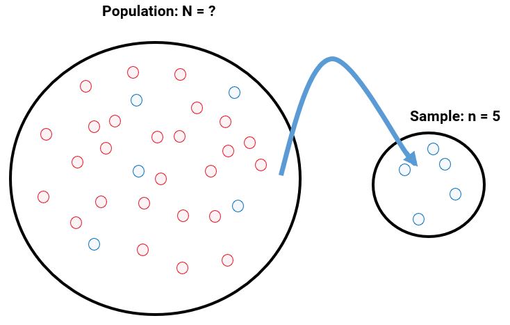
The above picture illustrates what is happening when we take a sample from a population. The population will have some number, \(N\), of units (these may be people or other members, elements, or subjects). Often, we don't know how many units a population consists of. We can then take a sample of \(n\) units - in the above diagram, we have \(n=5\). Often, samples are chosen randomly. We will learn more about sampling methods later on in this subject.
When we take a sample, we are hopeful that it is representative of the population. Considering the Breaking Bad example again, we estimated from our random sample that the average views per episode in earlier and later seasons were 1.398m and 1.866m respectively. But, we could take another random sample, and end up with different estimated average views per episode: for example, 1.336 and 2.996 respectively. In fact, every time we take a random sample, we could end up with a different estimate(s). How close are each of these sample estimates to the true population averages? We will usually never know - but Statistics gives us the tools to factor the uncertainty into our conclusions. This involves making use of probability models. We will be learning more about probability models and sampling distributions later on in this subject.