Week 2 Probability and Likelihood
In this material, we will visualize probability and likelihood functions using a specific example (i.e., a coin flip). Before we begin, please set up the environment:
- Change your working directory to Desktop/CM_course (or any preferred folder name).
- Open an R script and save it as Week2_[First and Last name].R in the current folder.
- Add a few comments to the first few rows of your R script. These comments will help you easily recall why and how to use this script. For instance:
# Week 2: Probability and Likelihood
# First and Last name
# date
- Last, tidy up the working environment panel. This helps prevent mistakes and makes it easier to find the variables in the Environment panel (Top-Right).
# clear working environment panel
rm(list=ls())
From now on, you can copy and paste my code to your own R script.
Run them (line-by-line using Ctrl+Enter in Windows/Linux or Command+Enter in Mac) and observe changes in the Environment panel (Top-Right) or Files/Plots (Bottom-Right).
Also, if you have time, you are encouraged to replace some variables’ values in the code and see how the results are changed.
2.1 Probability functions
A probability function, denoted as P(x), is a function used to assigns probabilities to the possible values of a random variable (X; which is used to quantify the outcome of the experiment). Here, when the possible values of a random variable is discrete, the probability mass function (PMF) is used. In contrast, we use the probability density function (PDF) to describe the probability distribution of continuous variable.
2.1.1 Probability mass function (PMF)
Imagine that you flip a fair coin once and your are recording the number of getting Head-side (H). In this example, what is your random variable?
The random variable (X) is either 1 or 0 when the Head-side is labeled as 1 and tail-side is labeled as 0.
With these details: the number of flips (N=1), random variables (1 or 0), theoretical probability of observing Head side (θ = 0.5), you can
1. draw a Probability Mass Function (PMF)
2. draw a Cumulative Mass Function (CMF)
3. sample a data from the PMF.
2.1.1.1 draw PMF using dbinom
dbinom is the function used to generate probability mass function for binomial distribution (i.e., the experiment with exactly two mutually exclusive outcomes of a trial.)
# See how to use dbinom. (e.g., what inputs are needed and what outputs are produced)
?dbinom
# According to the explanation provided by R. Three inputs are needed and should be put in the correct order to generate P(X=x):
# 1. x = Targeted value(s) of random variable (e.g., number of Head-side)
# 2. N = Number of attempts
# 3. θ = The theoretical probability of success (e.g., getting Head side)
P.Head <-dbinom(1, size = 1, prob = 0.5) # this code is equivalent to P(X = 1 | N=1, θ = 0.5)
P.Tail <-dbinom(0, size = 1, prob = 0.5) # this code is equivalent to P(X = 0 | N=1, θ = 0.5)You can also produce probabilities for all random variables by one click.
# produce probabilities for all random variables
N <- 1  # number of attempts
x <- 0:N # number of Head-side (from 0 to maximum: number of attemps).
theta <- .50 # theoretical probability of getting H
f <- dbinom(x, N, theta) # probability mass function
# Tip: Determine parameters before using the R function. By this way, you can
# - easily track them before you use them;
# - easily change parameters and see the results
With probability and values of a random variable, we can draw a PMF
#Visualize PMF of flipping a fair coin once
plot(x, f, type="h", xlab="x (number of Heads)", ylab="PMF",
        main="Binomial, N=1, theta=.50", xaxt="n")
# improve the quality of figure
points(x, f, pch=16) # check the usage
xtick<-seq(0, 1, by=1)
axis(side=1, at=xtick, labels = FALSE)
text(x=xtick,  par("usr")[3],
     labels = xtick, srt = 0, pos = 1, xpd = TRUE)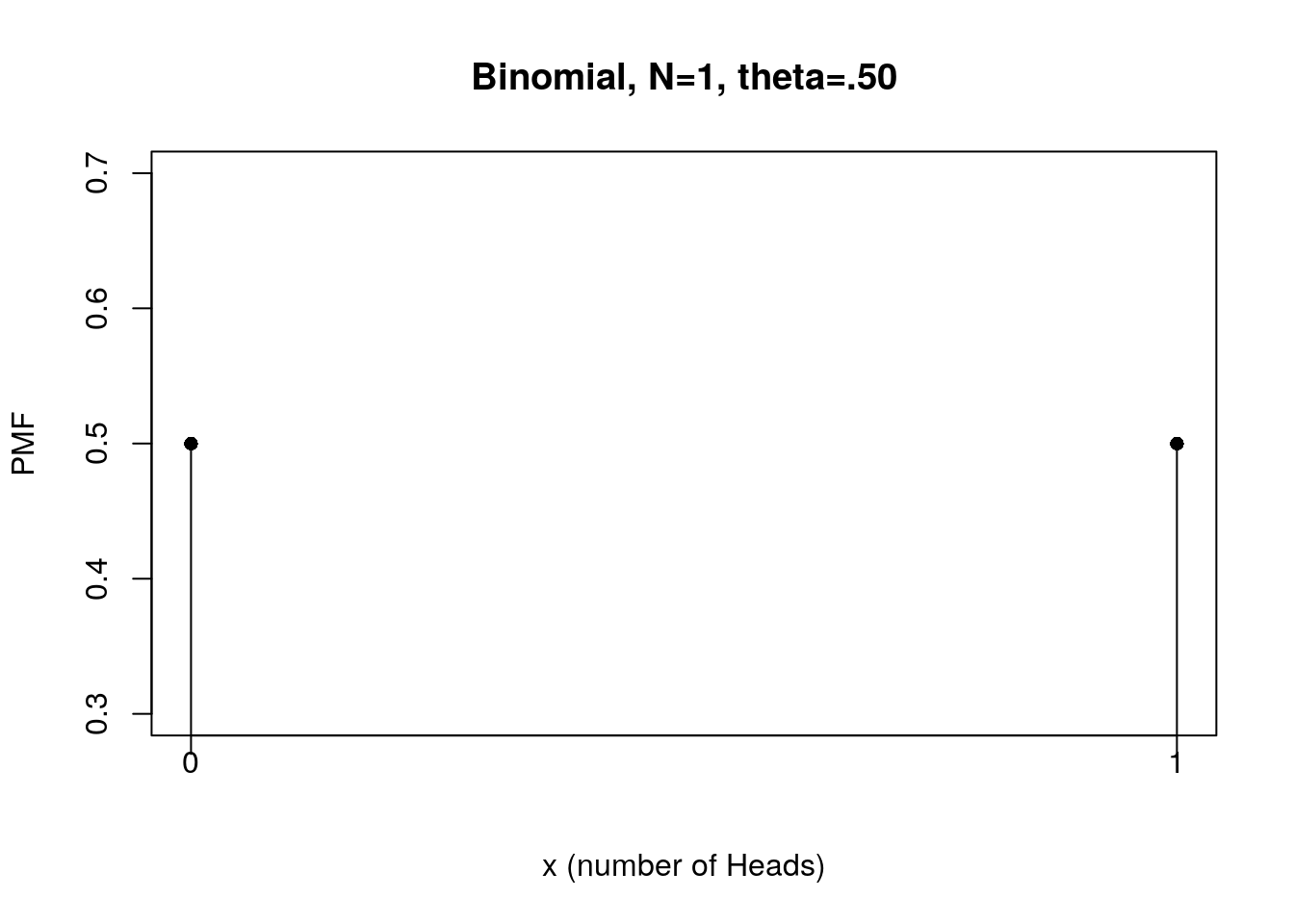
2.1.1.2 draw CMF using pbinom
Use pbinom to draw CMF. What are the required inputs? Same or different from the use of dbinom?
# See how to use pbinom
?pbinom
Apparently, we also need x, N and θ.
# We have created x, N, theta in the previous code. These objects are saved automatically in the environment. See the assigned value(s) by calling them.
x
N
theta
# Accumulate probabilities from x= 0 to x = 1
f.CMF <- pbinom(x, N, theta) # cumulative function
f.CMF## [1] 0.5 1.0
In a similar fashion we draw a CMF of x
#Visualize CMF of flipping a fair coin once
plot(x, f.CMF, type="h", xlab="x (number of Heads)", ylab="CMF",
        main="Binomial, N=1, theta=.50", xaxt="n")
# improve the quality of figure
points(x, f.CMF, pch=16) # check the usage
xtick<-seq(0, 1, by=1)
axis(side=1, at=xtick, labels = FALSE)
text(x=xtick,  par("usr")[3],
     labels = xtick, srt = 0, pos = 1, xpd = TRUE)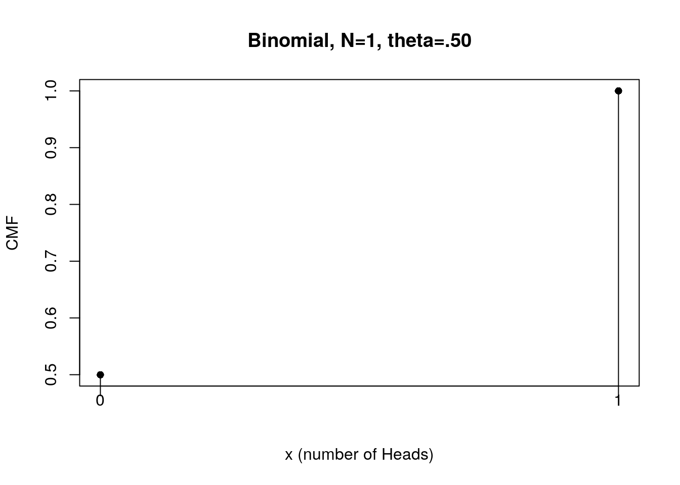
Now, make a comparison between PMF and CDF. What did you observe?
2.1.2 Exercise
2.1.2.1 Task A:
Suppose you are interested in PMF of tossing a fair coin 20 times. What are the possible outcomes now? Produce PMF and CMF for this example.
Hint: Now you just need to change one input mentioned in the course, so that you can quickly produce PMF and CMF!!
Discuss with your teammates which parameter should be changed?
Ideally, from the results of exercise, you can easily identify the features of binomial distribution and probability function:
1. As N increased to 20, the relative frequency of H peaks at θ × N.
2. The sum of probability of all possible events is 1.
3. The cumulative function is increased to 1.
2.1.2.2 Task B:
Compute the P(5≤x≤10), i.e., the probability of observing 5, 6, 7, 8, 9, 10 Heads for Binomial(N=20, θ=0.5).
Method1: Use the combination of dbinom() and sum()
Method2: Use pbinom() to compute P(x≤10)-P(x<5)
(Hint: use ? to understand what inputs and order of inputs for dbinom and pbinom.)
2.1.2.3 Task C (Generate data):
We are going to flip a coin 20 times in an experiment. Here we will run the experiment 100 times. Try to identify missing elements and complete the code below:
# 0. save known values
N <-   #number of repetitions  (One missing value)
n <-   #number of coin-flip in an experiment  (One missing value)

# 1. Create a sequence of number from 1 to 100. each number represents a repetition number.
Repetition.Number <- seq(from = ,to = N, by =1)   #(One missing value)
Repetition.Number
# 2. possible outcomes of each coin-flip: H and T. Create a vector contains H and T
outcome <- c() #(something is missing)
outcome
# 3. pre-determine a variable (e.g., mymat) and its size (of 100 rows for 100 experiments and 20 columns for 20 times of coin-flip in an experiment)
mymat  = matrix(nrow= , ncol= ) #(Two missing values)

# 4. Use for loop to sample and save data for each experiment
for (R in Repetition.Number){
mymat[] <- sample(outcome, ,replace = TRUE)} # flip a coin 20 times with replacement  (two missing elements; check index of mymat and ?sample)
#open mymat in Environment window and see what you created

# 5. compute the numbers of observing Head-side in each experiment
myFreq <- rowSums(mymat == ) #(One missing value)

# 6. Use table() to compute the frequency of observing 1, 2, 3, ..., 10 Head-side
table(myFreq)

# 7. visually inspect the result (distribution) and tell us the peak of relative frequency. What does it mean?
2.1.3 Generate data
Unlike dbinom and pbinom directly return the probability of the event of interest, we generate our own data given information about the experiment In the Task C. This can be done by using rbinom to sample data from the Binomial distribution.
# check how to use rbinom
?rbinom
Unlike dbinom and pbinom runs an experiment once (with 1 or 20 trials), rbinom repeats the same experiment with N trials r times.
# set up inputs
nRepeat <- 10 # number of repetition.
N <- 20  # number of attempts
theta <- .50 # theoretical probability of getting H
# sample data given information.
data <- rbinom(nRepeat, N, theta)
data # data stores number of Heads in each repetition of tossing a coin N times## [1] 11 11 11 8 8 7 10 7 5 13Let’s calculate probability of each event with table().
frequency <- table(data) # table() helps us to summarize the frequency of each event
Prob.event <- frequency/nRepeat # compute probability given frequency and repetitions
Prob.event
## data
## 5 7 8 10 11 13
## 0.1 0.2 0.2 0.1 0.3 0.1Does it look like the figure you produce in the Exercise?
Now let’s try the same code BUT increase the number of repetition from 10 to 10000.
nRepeat <- 10000 # number of repetition
N <- 20  # number of attempts
theta <- .50 # theoretical probability of getting H
data <- rbinom( nRepeat, N, theta)
frequency <- table(data)
Prob.event <- frequency/nRepeat
Prob.event
## data
## 3 4 5 6 7 8 9 10 11 12 13
## 0.0006 0.0048 0.0152 0.0361 0.0737 0.1231 0.1568 0.1802 0.1639 0.1194 0.0713
## 14 15 16 17 18
## 0.0352 0.0142 0.0045 0.0009 0.0001# Plot the histogram for this sample.
plot(Prob.event)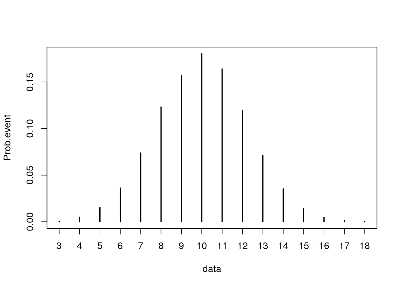
2.2 Likelihood
A probability of an random variable x is determined by θ and N. In contrast, likelihood denotes how likely θ is true given x and N.
The relationship between probability and likelihood can be found in there equations.
Probability mass function: P(x|θ,N)
likelihood function: LF(θ) = P(θ|x,N).
2.2.1 Likelihood function (LF)
Two similar methods can be used to illustrate it:
Method 1: Using bdinom and fix x, N but varies θ.
(Remember!! “The likelihood involves exactly the same function as the probability density, but use it for a different purpose” Farrell & Lewandowsky, 2018. Ch4.)
x <- 10
N <- 20
LF.theta <- seq(0, 1, 0.0001) # a vector of possible thetas
f <- dbinom(x, N, LF.theta) # see how probability of a certain event is changed as function of theta: fix x, N but varies θ.
plot(LF.theta, f, type="l", xlab="θ", ylab="LF", main="P(θ |x=10, N=20)")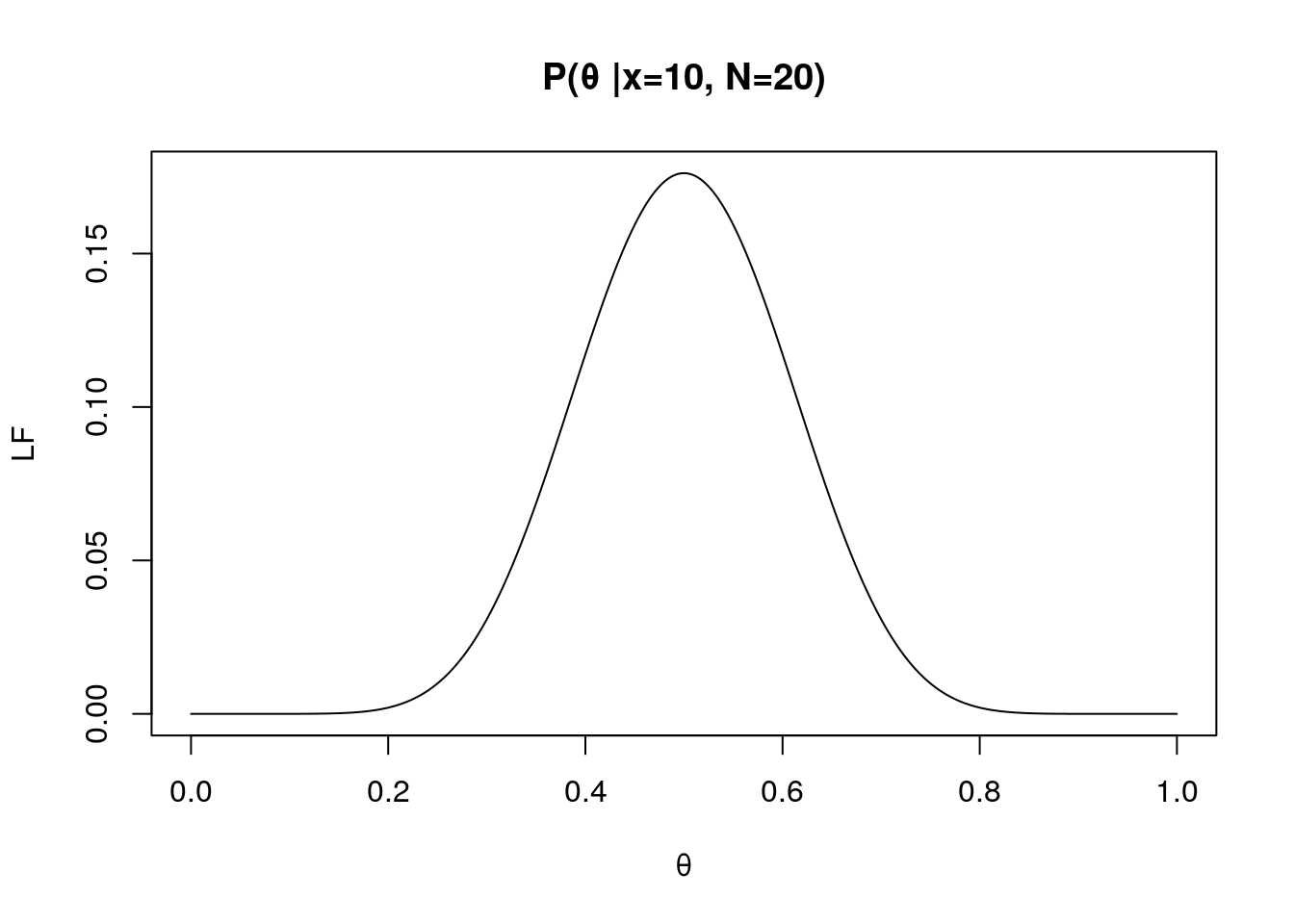
Method 2: Create a function named LF and use x, N and θ as inputs. This method is basically equivalent to the first method.
# Create a LF function
# inputs: theta, x and N
# output: Likelihood
LF <- function(LF.theta,x,N){
  dbinom(x,N,LF.theta) }

# Set up the inputs for LF you created
# The most important thing is "varying probability of success on each trial"
x <- 15
N <- 20
LF.theta <- seq(0, 1, 0.0001) # varied probability of success
f <- LF(LF.theta, x, N)

# plot the likelihood as function of probability of success
plot(LF.theta, f, type="l", xlab="θ", ylab="LF", main="P(θ |x=15, N=20)")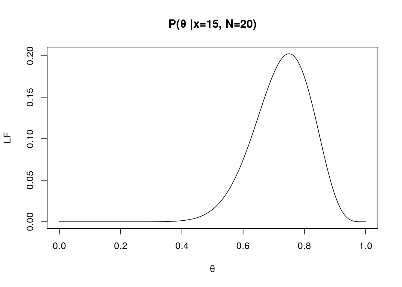
2.2.2 Maximum likelihood
In the figure right above, the highest likelihood can be found around θ = 0.75. This is known as maximum likelihood of θ.
The maximum likelihood of θ is changed given number of observing Heads and number of attempts.
For instance, if you only observed 10 Heads over flipping a fair coin 20 times, then the maximum likelihood of θ is 0.5.
x <- 10
N <- 20
LF.theta <- seq(0, 1, 0.0001)# a vector of possible thetas
f <- LF(LF.theta, x, N)
plot(LF.theta, f, type="l", xlab="θ", ylab="LF", main="LF, x=10, N=20")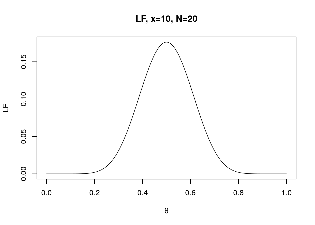
Overall, you should be able to observe the changes in maximum likelihood as which maximum likelihood of θ always found at x/N. In other words, θ is likely to be 0.5 if you observe 10 Heads over 20 flips; θ is likely to be 0.75 if you observe 15 Heads over 20 flips.
2.2.3 Interpretation of likelihood ratio
The probability function assumes that you know the actual probability of getting Heads or being success. However, in most case we only know the outcomes. For instance, 15 Heads over flipping a coin 20 times and we don’t know whether the coin is fair or not.
In this case, how do we know if the probability of getting Heads side or being success is 0.5 or 0.75? The likelihood ratio will tell you which one is more likely happen.
#compute likelihood for each hypothesis given computed LF
LF50 <- LF(0.5, 15, 20)
LF75 <- LF(0.75, 15, 20)
LF50
## [1] 0.01478577LF75## [1] 0.2023312The results 0.0147 and 0.2023 indicate that you are likely to observe 15 Heads if the probability of getting Heads is 0.75
#compute Likelihood ratio (LR)
LFratio <-LF75/LF50
LFratio
## [1] 13.68418The value of 13.68 indicates that your data is 13.68 times more likely to be observed when θ = 0.75 than when θ = 0.5. The result also implies that hypothesizing θ = 0.75 is better to explain data.
2.2.4 (Additional Materials) Test Binomial outcome
- Using Binomial test:
# simulate data 10000 times given fixed X and N and then test the hypothesis (θ=0.5)
N <- 20
X <- 15
nSimulation <- 10000
simul_data <- rbinom(nSimulation, N, 0.5)
# test with binomial test
binom.test(X, N, 0.5, alternative = "greater")##
## Exact binomial test
##
## data: X and N
## number of successes = 15, number of trials = 20, p-value = 0.02069
## alternative hypothesis: true probability of success is greater than 0.5
## 95 percent confidence interval:
## 0.5444176 1.0000000
## sample estimates:
## probability of success
## 0.75- Based on LR
LR <- LF(.75, X, N)/LF(.50, X, N)
simul_LRs <- LF(.75, simul_data, N)/LF(.50, simul_data, N)
mean(simul_LRs >= LR)
## [1] 0.0212.3 Normal distribution
Suppose your possible events are continuous variables (e.g., reaction time), then the random variable contains infinite elements because you can always find a number between two values?
From this view, can we find the probability of specific RT, for example, RT=4 (i.e., P(RT=4))?
The answer is NO. Recall the properties of probability density function (PDF): The probability an observation on a continuous variable is 0. Therefore, it implies that the probability of observing exact RT of 4.0000s approximates 0.
# call description of dnorm in Help window (bottom-right)
?dnorm
From the help function, you can see that the inputs are mean, standard deviation and a vector of numbers.
For instance: dnorm(x, mean = 0, sd = 1)
2.3.1 draw PDF using dnorm
x <- seq(-4, 4, 0.01) # create a sequence of numbers from -4 to 4 stepping by 0.01
Mu  <- 0 # theoretical mean
Std <- 1 # theoretical stander deviation
norm.PDF <- dnorm(x, Mu, Std) # theoretical stander deviation

plot(x, norm.PDF, xlab="x", ylab="PDF",
        main="Normal, Mu =0, std = 1")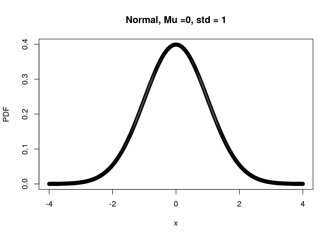
Recall the properties of probability again and look at the figure your plotted right above, do you observe any strange pattern?
The summed probability across random variable is larger than 0?! Does R make any mistake?
No, each dot on the figure represent “Density” rather than a probability of exact data point (e.g., x = 3.0000). In the other words, if you are interested in P(X=3), the answer is 0 but R returns P(X=3±errors) here.
In this case, each data point reflects not only its own probability but also errors’ probability.
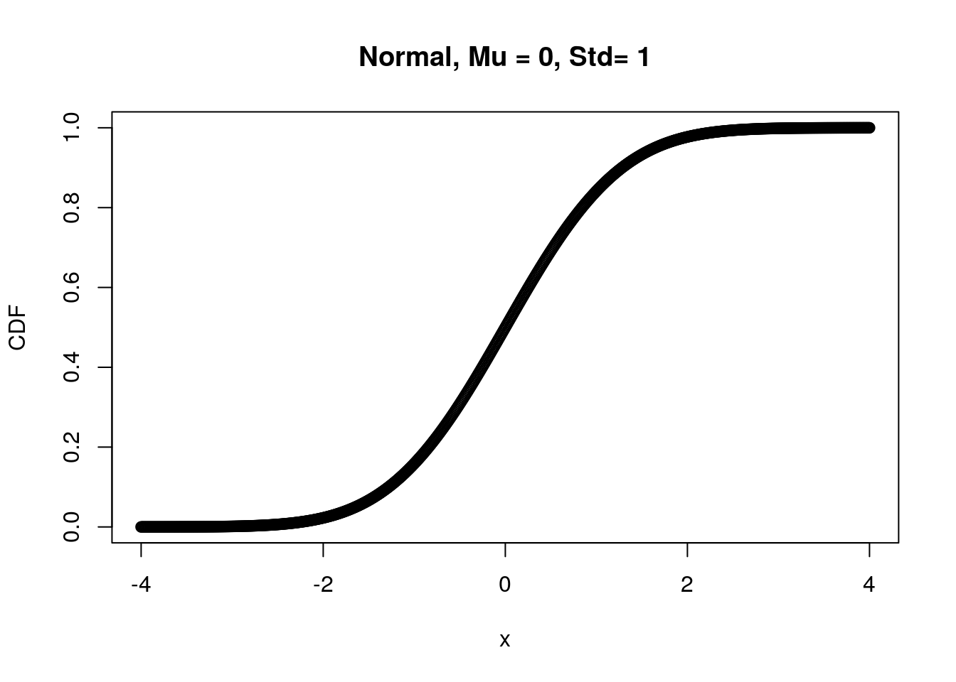
This is not the issue when we accumulate density from low to high values of a random variable in the cumulative function.
2.4 Exercise
2.4.3 Task F:
A normal distribution with mean = 400 and SD = 100, what is the probability of getting numbers between 10 and 300 (inclusive)?
2.4.4 Task with Dice rolls:
http://ditraglia.com/Econ103Public/Rtutorials/Rtutorial4.html#dice-rolls-with-sample
2.5 Answers
2.5.1 Task A
# Flip a fair coin 20 times, so the N (number of trials) should be 20 rather than 1
N <- 20  # number of attempts
x <- 0:N # number of H observations or let's say random variables
theta <- .5 # theoretical probability of getting H
f20 <- dbinom(x, N, theta) # probability mass function
plot(x, f20, type="h", xlab="x", ylab="PMF",
        main="Binomial, N=20, theta=.90")
points(x, f20, pch=16)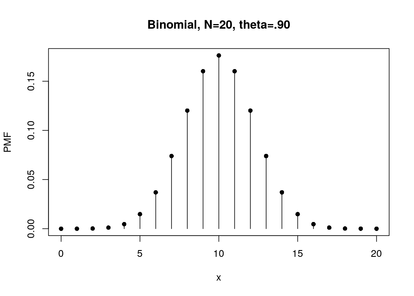
# CMF for the case of Flipping a fair coin 20 times
f20.CMF <- pbinom( x, N, theta)
plot(x, f20.CMF, type="h", xlab="x", ylab="CMF",
        main="Binomial, N=20, theta=.50")
points(x, f20.CMF, pch=16)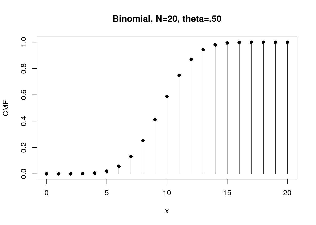
2.5.2 Task B
#Method1: Use the combination of `dbinom()` and `sum()`
N <- 20
theta<-0.5
x.lower <- 5
x.higher<-10
x.interest<-x.lower:x.higher  #or x.interest = seq(x.low,x.high,1)
p.individual<-dbinom(x.interest,N,theta)
p.accumulate<-sum(p.individual)
p.accumulate
## [1] 0.5821896#Method2: Use `pbinom()` to compute P(x≤10)-P(x<5). Note: the x = 5 should be included
x.LExclude<-4
x.HInclude<-10
p.low<-pbinom(x.LExclude,N,theta)
p.high<-pbinom(x.HInclude,N,theta)
p.range<-p.high - p.low
p.range## [1] 0.5821896# the results from method 1 and method2 should be the same.2.5.3 Task C:
# 0. save known values
N <- 100 #number of repetitions
n <- 20  #number of coin-flip in an experiment

# 1. Create a sequence of number from 1 to 100. each number represents a repetition number.
Repetition.Number <- seq(from = 1,to = N, by =1)
Repetition.Number
## [1] 1 2 3 4 5 6 7 8 9 10 11 12 13 14 15 16 17 18
## [19] 19 20 21 22 23 24 25 26 27 28 29 30 31 32 33 34 35 36
## [37] 37 38 39 40 41 42 43 44 45 46 47 48 49 50 51 52 53 54
## [55] 55 56 57 58 59 60 61 62 63 64 65 66 67 68 69 70 71 72
## [73] 73 74 75 76 77 78 79 80 81 82 83 84 85 86 87 88 89 90
## [91] 91 92 93 94 95 96 97 98 99 100# 2. possible outcomes of each coin-flip: H and T. Create a vector contains H and T
outcome <- c('H','T')
outcome## [1] "H" "T"# 3. pre-determine a variable (e.g., mymat) and its size (of 100 rows for 100 experiments and 20 columns for 20 times of coin-flip in an experiment)
mymat = matrix(nrow=N, ncol=n)
# 4. Use for loop to sample and save data for each experiment
for (R in Repetition.Number){
mymat[R,] <- sample(outcome,20,replace = TRUE)} # open mymat in Environment window and see what you created
# 5. compute the numbers of observing Head-side in each experiment
myFreq <- rowSums(mymat == 'H')
# 6. Use table() to compute the frequency of observing 1, 2, 3, ..., 20 Head-side
table(myFreq)## myFreq
## 3 5 6 7 8 9 10 11 12 13 14 15
## 2 2 3 11 12 10 17 15 13 6 8 1# 7. visually inspect the result (distribution) and tell us the peak of relative frequency. What does it mean?2.5.4 Task D:
x <- 150
N <- 750
LF.theta <- seq(0, 1, 0.0001)
f <- dbinom(x, N, LF.theta) # see how probability of a certain event is changed as function of theta: fix x, N but varies θ.
plot(LF.theta, f, type="l", xlab="θ", ylab="LF", main="LF, x=150, N=750")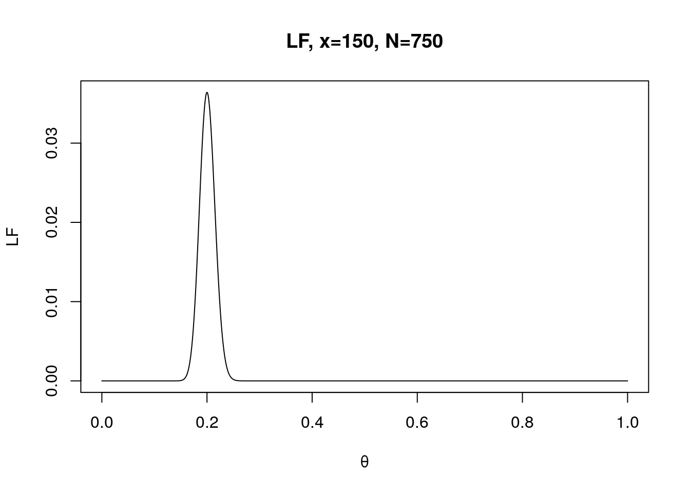
2.5.5 Task E:
x <- seq(from = -100, to = 900, 0.01)
Mu  <- 400 # theoretical mean
Std <- 100 # theoretical stander deviation
TaskE.PDF <- dnorm(x, Mu, Std) # theoretical stander deviation

plot(x, TaskE.PDF, xlab="x", ylab="PDF",
        main="Normal, Mu =400, std = 100")

# add color to the region of interest
x2 <- seq(200,300,0.01) # from 10 to 300 increased by 0.01
y2 <-  dnorm(x2, Mu, Std)
x2 = c(200,x2,300)
y2= c(0,y2,0)
polygon(x2,y2, col="yellow", border=NA)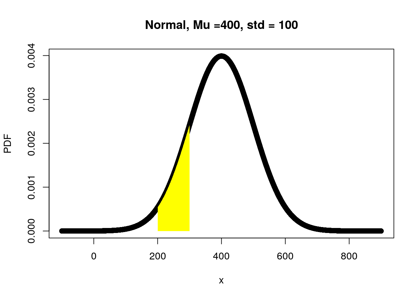
2.6 Wrap up and Preview
- Add
?before any build-in R function (e.g.,?plot) to understand how to use it and what output is. - We haven’t run the “Cognitive models” yet, but we have tried something similar. That is, we simulated/generated “fake” data given inputs (x, N, θ) and probability functions.
- We will simulate more data with cognitive models next week.