Week 1 R basic

1.1 Learning objects

Familiarize yourself with R scripts;
Gain confidence in translating equations into scripts/functions.

1.2 Introduction

This week, you will learn basic R functions, including calculations (e.g., +, -, x, /), loops, and logical operations, commonly used in transforming equations into programming language. In addition to these functions, you need to understand the meaning of each notation in the equation and where to find the values for each notation. Usually, this information is explicitly described in the paper. Let’s set aside cognitive models for now and use a well-known equation for z-scores: \[ Z = \frac{x_i - \bar{x}}{\sigma} \]
Here, x refers to each data point i, $\bar{x}$ refers to the mean of all data points and $\sigma$ indicates the standard deviation of data. Without using R’s build-in functions (like mean() and sd()), can you translate this equation into code (see Task B for details)?
*** Notice: If you know of a valid sharing code/function in R, you can always use it directly instead of writing your own. The practice without using R’s built-in functions aims to give you an understanding of how equations are transformed into programming language. Once you can write your own function, you won’t need to worry if some equations/models haven’t been transformed into codes. Moreover, you’ll gain a deeper understanding of how the equation works.

1.3 Before you start…

If you are not familiar with R or are using R for the first time, please start from sections 1.1 and 1.2. In these two subsections, we will cover common settings when you start using R to analyze data and basic R functions, including calculations (e.g., +, -, x, /), loops, and logical operations.

If you are familiar with R or frequently use it to analyze data, you can try Tasks A-E and assist team members if they have any questions.

1.4 R environment & setup working space

Imagine you have a dataset at hand and you’d like to use R to organize and analyze it.
Follow the steps below to set up the R environment and explore R:
1. Install R AND RStudio: If you haven’t already, download and install R from CRAN and RStudio from RStudio’s website.
2. Open RStudio: Once installed, open RStudio and you will see something like Figure 1.1

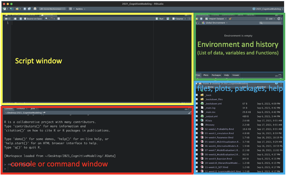
Figure 1.1: Create and save script

1.4.1 Change your working directory

In this course, save your scripts in the directory ~/Desktop/CM_course. To do so, follow these steps:
1. Create a folder named CM_course (or any preferred folder name) on your desktop.
2. Return to RStudio and check your current working directory by executing getwd() in the R Console. If you’re unsure how to do this, copy (or type) the code below and paste it into your Console window after the prompt >:
3. Press Enter to run the code, and you will see the current working directory displayed in the Console.

# Type getwd() in your Console window to know the current working directory.
getwd()

## [1] "/opt/rstudio-connect/mnt/report"

If the output does not end with the folder name where you intend to save your R script (e.g., Desktop/CMcourse), you can use setwd() to change the working directory. Alternatively, you can specify your working directory under Session-> set working directory -> Choose Directory.

Once you have completed these steps, type getwd() again in the Console window to verify if you have successfully changed your working directory.

Tip 1: You can also check the current working directory from the top of the console panel (see Figure 1.1, right).
Tip 2: If you want to open the same working directory every time you open R, go to Tools –> Global options and click on Browse to select the default working directory you prefer.
***Notice: Changing the working directory won’t synchronize the directory in the Files pane (i.e., the bottom-right panel). To synchronize the directory in the Files pane with the current working directory, click the arrow at the top-left of the Console window.

1.4.2 Create and Save your first script

The script is the simplest code file, which is used to store and run a sequence of commands.
1. Creat a R script: You can open a new R script from New File tap and save it as Week1_[First and Last name].R (e.g., Week1_Rbasic_ChihChungTing.R) in the current working directory (see Figure 1.2, top) by Command+S (for Mac) or Ctrl+S (for Windows).
*** Notice: If you successfully created a script, you should see one more file named Week1_[topic]_[First and Last name].R in your Files window (see Figure 1.2, bottom).

Now, let’s begin editing the script step-by-step together. We’ll save the exercises for today in the same script.

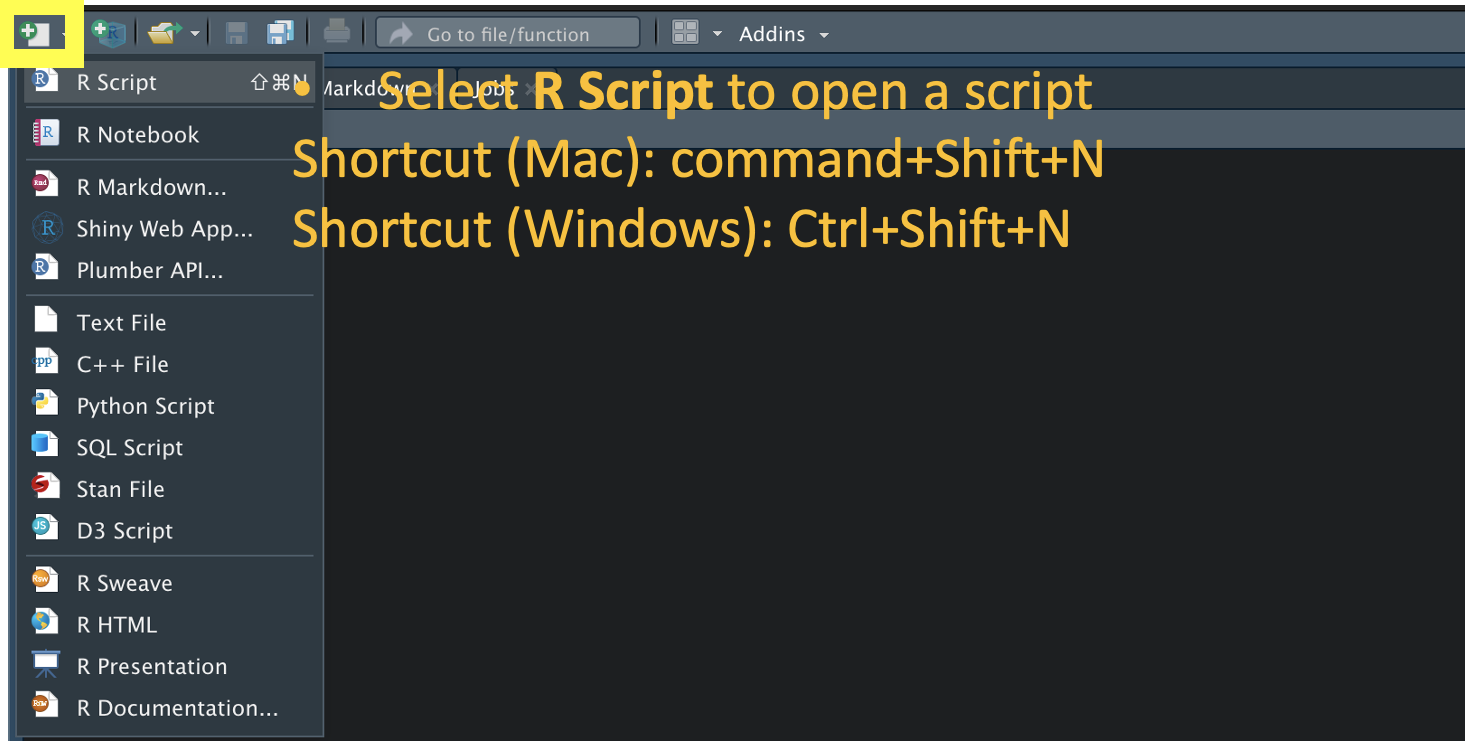
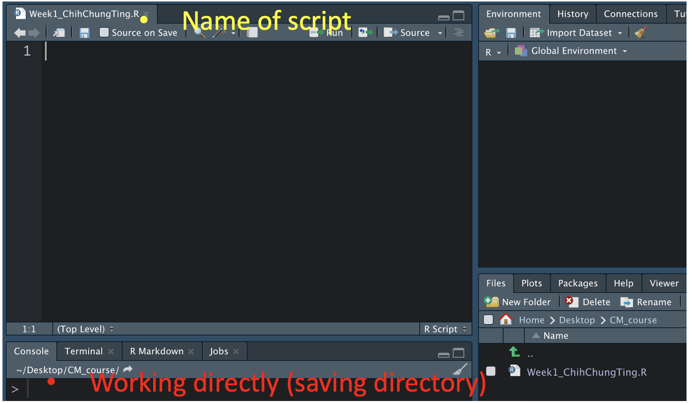
Figure 1.2: Create and save script

2. Begin by describing the script in the first few lines. Remember, lines starting with a hash sign # are typically used as comments to remind you of the purpose of the codes/scripts. We usually use the first few lines in a script to describe the general information (e.g., why and when did you create this script? how to use the script?).

# Week 1: R basics 
# Your First and Last name
# date

3. Clean up the Environment window by typing rm(list = ls()) in your script.
The line(s) in a script can be run by
- highlighting the line(s) you want to run and
- pressing Command+Enter or Ctrl+Enter

# clean up the Environment window
rm(list = ls()) # select this line and press command+Enter or Ctrl+Enter to execute it

4. Load data from csv file and look at the first six rows. (Data stored in different types of files, including .Rdata, .txt, .xls and .csv, can be loaded. Now, try the code below in your script and run it by select them and press Command+Enter or Ctrl+Enter.
*** Notice: Use # to explain the meaning of each variable.

# Load data from Why do we overestimate others' willingness to pay? Matthews, W. J., Gheorghiu, A. I., & Callan, M. J. (2016)
# brief introduction to the dataset: 
# task: Participants were randomly assigned either to “estimate the proportion of people taking part in the survey who have more money than you do” (coded 1) or the proportion who “have less money than you do” (coded 0), and typed their estimate in a text box. For each of 10 product (p1-p10), the participant indicated whether the amount they would be willing to pay is more or less than what “the typical person taking this survey today would be willing to pay” (product order and left-right assignment of the “less” and “more” response options were randomized).
# id: participant id code
# gender: participant gender. 1 = male, 2 = female
# age: participant age
# income: participant annual household income on categorical scale (see main text of paper)
# p1-p10: Participants indicated whether the amount that they would be prepared to pay for each of 10 products was more (code 1) or less (code 0) than what the typical person would pay.
# pcmore: participant's estimate of the proportion of people who have more than they do (calculated as 100-haveless when task=0)

# Method 1 (might be terminated by SSL connect issue. If this is the case, try Method 2)
data<-read.csv("http://journal.sjdm.org/15/15909/data1.csv")
head(data)

##                  id gender age income p1 p2 p3 p4 p5 p6 p7 p8 p9 p10 task
## 1 R_3PtNn51LmSFdLNM      2  26      7  1  1  1  1  1  1  1  1  1   1    0
## 2 R_2AXrrg62pgFgtMV      2  32      4  1  1  1  1  1  1  1  1  1   1    0
## 3 R_cwEOX3HgnMeVQHL      1  25      2  0  1  1  1  1  1  1  1  0   0    0
## 4 R_d59iPwL4W6BH8qx      1  33      5  1  1  1  1  1  1  1  1  1   1    0
## 5 R_1f3K2HrGzFGNelZ      1  24      1  1  1  0  1  1  1  1  1  1   1    1
## 6 R_3oN5ijzTfoMy4ca      1  22      2  1  1  0  0  1  1  1  1  0   1    0
##   havemore haveless pcmore
## 1       NA       50     50
## 2       NA       25     75
## 3       NA       10     90
## 4       NA       50     50
## 5       99       NA     99
## 6       NA       20     80

# Method 2(if Method1 doesn't work)
# Download the data1.csv via the link https://www.dropbox.com/s/ykyl6iio4j26p9g/data1.csv?dl=0
# save the data1.csv in /Desktop/CM_course  
# type following lines (without #) in your console window and run them:
# data<-read.csv("~/Desktop/CM_course/data1.csv") # replace the directory if you save data1.csv in other place.
# head(data)

Look into data closely via View(data), which directly open data in the new tap. Alternatively, use data$ and then press Tab. You will see all available variable names in data.

# Look into data closely
data$age # specifically look into or select values/characters in Age

##   [1] 26 32 25 33 24 22 47 26 29 32 29 28 31 24 25 28 20 41 44 23 49 26 19 57 30
##  [26] 25 26 60 32 29 29 44 40 28 25 32 31 27 31 44 31 27 26 28 22 39 51 34 22 25
##  [51] 37 59 18 33 26 67 30 35 34 34 20 42 37 20 28 24 45 25 44 46 29 37 31 42 25
##  [76] 33 43 25 21 23 34 30 31 24 24 35 29 33 53 38 32 22 30 26 31 32 29 41 21 28
## [101] 49 22 28 27 30 41 26 31 22 45 27 27 37 26 23 26 29 28 22 44 25 49 21 27 37
## [126] 23 55 33 38 28 48 37 34 25 29 41 21 38 38 32 30 27 23 29 28 24 22 52 32 22
## [151] 23 30 31 34 24 32 34 39 30 25 31 20 33 31 24 36 24 24 30 29 26 26 57 40 36
## [176] 28 24 31 34 33 58 24 44 23 25 33 23 33 23 29

data$income # specifically look into or select values/characters in Income

##   [1] 7 4 2 5 1 2 3 4 1 7 4 3 2 2 6 3 2 2 1 3 3 6 4 5 5 2 3 2 5 4 6 7 5 1 5 2 4
##  [38] 4 5 6 4 2 2 4 6 1 8 6 2 4 4 4 6 1 6 2 5 4 3 2 4 1 6 2 2 1 4 5 5 5 1 6 5 6
##  [75] 2 1 7 4 5 8 2 3 2 1 6 4 4 1 2 4 5 4 2 6 1 3 5 2 5 5 2 3 4 2 3 7 8 3 1 2 1
## [112] 1 4 6 2 6 3 5 5 1 6 6 3 6 4 5 7 2 4 2 2 3 3 4 4 2 1 6 2 2 5 4 1 3 1 2 1 3
## [149] 1 1 2 3 6 5 3 5 5 2 2 3 1 3 5 2 5 2 2 2 3 3 2 4 5 6 5 1 4 1 7 3 6 1 2 3 3
## [186] 2 2 6 2 6

Now, type data$pc and then press Tab. What do you see?

1.5 Basic R functions

Here, we will use the imported data [Matthews, W. J., Gheorghiu, A. I., & Callan, M. J., 2016, Why do we overestimate others’ willingness to pay?] (http://journal.sjdm.org/15/15909/jdm15909.pdf) to learn basic R functions.
If you are familiar with R functions, it is still recommended to go through the materials. Boring? Solve tasks in the Exercises section and helps your teammates to debug (debugging is an important skill!).

1.5.1 Calculators

R is able to handle many basic calculation (+, -, x, /).
1. Sum up values from two selected columns

# 1. Sum
data$p1+data$p2 # sum of p1 and p2

##   [1] 2 2 1 2 2 2 2 2 2 2 2 2 0 2 1 1 2 2 2 2 1 0 2 1 1 2 1 2 1 2 2 1 2 2 2 2 2
##  [38] 2 2 2 0 1 2 2 1 1 2 2 2 1 2 1 2 2 1 1 1 2 2 1 1 2 2 1 2 2 2 1 2 2 2 1 1 0
##  [75] 2 2 2 2 2 2 2 1 1 2 1 2 2 2 2 1 1 1 1 1 2 1 0 2 0 2 2 2 2 1 2 2 2 2 1 2 2
## [112] 2 2 1 1 0 2 1 2 2 0 2 2 1 2 2 2 2 1 2 2 2 1 1 2 2 2 2 2 1 2 1 2 1 2 2 2 2
## [149] 1 2 2 1 0 2 1 2 2 2 2 1 2 0 1 1 1 2 0 0 1 2 2 1 2 2 2 1 2 2 1 2 1 2 0 1 2
## [186] 2 2 1 2 2

2. Subtract a certain number. For example, you want to know the subjects’ birth year.

# 2. Subtraction
2021-data$age # To backtrack the birth year, use current year - age to identify it.

##   [1] 1995 1989 1996 1988 1997 1999 1974 1995 1992 1989 1992 1993 1990 1997 1996
##  [16] 1993 2001 1980 1977 1998 1972 1995 2002 1964 1991 1996 1995 1961 1989 1992
##  [31] 1992 1977 1981 1993 1996 1989 1990 1994 1990 1977 1990 1994 1995 1993 1999
##  [46] 1982 1970 1987 1999 1996 1984 1962 2003 1988 1995 1954 1991 1986 1987 1987
##  [61] 2001 1979 1984 2001 1993 1997 1976 1996 1977 1975 1992 1984 1990 1979 1996
##  [76] 1988 1978 1996 2000 1998 1987 1991 1990 1997 1997 1986 1992 1988 1968 1983
##  [91] 1989 1999 1991 1995 1990 1989 1992 1980 2000 1993 1972 1999 1993 1994 1991
## [106] 1980 1995 1990 1999 1976 1994 1994 1984 1995 1998 1995 1992 1993 1999 1977
## [121] 1996 1972 2000 1994 1984 1998 1966 1988 1983 1993 1973 1984 1987 1996 1992
## [136] 1980 2000 1983 1983 1989 1991 1994 1998 1992 1993 1997 1999 1969 1989 1999
## [151] 1998 1991 1990 1987 1997 1989 1987 1982 1991 1996 1990 2001 1988 1990 1997
## [166] 1985 1997 1997 1991 1992 1995 1995 1964 1981 1985 1993 1997 1990 1987 1988
## [181] 1963 1997 1977 1998 1996 1988 1998 1988 1998 1992

3. Mean and standard deviation of selected data (Hint: mean() and sd())

# 3. Mean and standard deviation
mean(data$age) # averaged age

## [1] 31.71579

sd(data$age) # standard deviation of age

## [1] 9.123101

4-5. Frequency distribution (Hint: table())

# 4. frequency 
table(data$gender) #frequency for each gender type

## 
##   1   2 
## 119  71

# the first row refers to categories
# the second row refers to frequency in a certain category

# 5. Division
table(data$gender)/length(data$id) #to calculate the percentage of each category

## 
##         1         2 
## 0.6263158 0.3736842

6-8. Other calculator functions:

# 6. Multiply
data$pcmore*0.01 # having more money than me (%)

##   [1] 0.50 0.75 0.90 0.50 0.99 0.80 0.95 0.70 0.70 0.25 0.50 0.50 0.56 0.80 0.35
##  [16] 0.95 0.50 0.98 0.85 0.15 0.45 0.25 0.75 0.50 0.50 0.70 0.45 0.25 0.65 0.50
##  [31] 0.10 0.50 0.40 0.50 0.80 0.90 0.60 0.50 0.30 0.50 0.40 0.75 0.60 0.70 0.70
##  [46] 0.25 0.50 0.10 0.90 0.55 0.60 0.50 0.90 1.00 0.40 0.90 0.60 0.60 0.60 0.85
##  [61] 0.90 0.70 0.98 0.70 0.60 0.75 0.80 0.50 0.60 0.80 0.90 0.80 0.70 0.30 0.80
##  [76] 0.90 0.40 0.70 0.70 0.00 0.60 0.20 0.85 0.20 0.50 0.96 0.80 0.70 0.02 0.70
##  [91] 0.70 0.40 0.80 0.70 0.75 0.30 0.40 0.90 0.60 0.40 0.70 0.50 0.80 0.60 0.25
## [106] 0.50 0.50 0.90 0.65 0.75 0.95 0.95 0.53 0.50 0.75 0.30 0.55 0.50 0.50 0.99
## [121] 0.25 0.40 0.85 0.40 0.75 0.45 0.25 0.93 0.60 0.75 0.65 0.70 0.70 0.40 0.30
## [136] 0.75 0.90 0.50 0.50 1.00 0.30 0.50 0.80 0.50 0.50 0.70 0.95 0.30 0.75 0.95
## [151] 0.60 0.85 0.50 0.65 0.85 0.50 0.50 0.80 0.65 0.60 0.20 0.80 0.45 0.95 0.55
## [166] 0.50 0.80 0.70 0.70 0.40 0.40 0.90 0.50 0.80 0.70 0.75 0.50 0.99 0.50 0.50
## [181] 0.50 0.85 0.85 0.30 0.50 0.25 0.50 0.40 0.60 0.35

# 7. Root square (sqrt())
sqrt(4)

## [1] 2

# 8. Power function (^)
3^2

## [1] 9

1.5.2 Assignment

Do you notice that all of outputs from above cannot be used for further analysis? Even though these outputs are visible in the Colsole window, you have to run the same code again to produce the output.
This is not the problem if you store outputs in a variable using = or <-.
Left-hand side of = or <- is the variable name and Right-hand side of = or <- is the assignment.
Good news: You can name variables based on your preference. Moreover, with assignment, you won’t see the output in the Console panel. This is helpful if you want to keep the console window as clean as possible.

Bad news: The same variable name will be replaced without any warning message. One possible solution is to use unique variable names to represent the assignments.
Let’s try two examples here:
Example1: Number of subjects.

# Example1: Number of subjects.
# If each row represents a subject, you can use R's built-in function nrow() or length() to check the number of rows and save it as the number of subjects (e.g., nSubj).
nSubj <- length(data$id) # or nSubj <- nrow(data)

# To see the results, type the name of variable.
nSubj

## [1] 190

Example2: Frequency distribution of gender

#Example2: Frequency distribution of gender
gender.frequency<- table(data$gender)
gender.percent <-gender.frequency/nSubj # Using variable created before to complete calculation!!!!
gender.percent

## 
##         1         2 
## 0.6263158 0.3736842

Bad news: The same variable name will be replaced without any warning message!!!

# the existing variable will be replaced by any new value(s) without any error or warning message!!!
gender.percent <- 0 
gender.percent

## [1] 0

1.5.3 Logical operations and index

R can also evaluate the logical statement. If the statement is correct, then output is TRUE, otherwise, FALSE. Here are few simple examples:

## Logical operations and index
#whether 100 is larger than 40?
 100>40

## [1] TRUE

# whether the names are the same?
"Kavin" == "Kevin"

## [1] FALSE

# which values in a vector are larger than 10?
x = c(11,12,3,4,5) # create a vector of numbers
x

## [1] 11 12  3  4  5

x>10

## [1]  TRUE  TRUE FALSE FALSE FALSE

Logical operations can be applied in various scenarios. For instance, in prospect theory (Kahneman & Tversky, 1979), the subjective perception of option utility is influenced by its valence. Specifically, gains and losses may be assessed differently (see Figure 1.3).

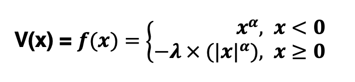
Figure 1.3: Value function

Conditional execution (Hing: if)

## logical operation: 
# Conditional execution: if statement is true then execute the code.
a <-100
b <- 10
if (a>b) {
print("Correct")}

## [1] "Correct"

# More complicated statement: if A AND B are true, then execute
if (50<a & 50>b) {
print("Two statements are true")}

## [1] "Two statements are true"

# More complicated statement: if A OR B is true, then execute
if (100<a | 100>b) {
print("One statement is true")}

## [1] "One statement is true"

Now, try to use what you have learned above to translate the equation of value function (Figure 1.3, top) into code. (Assume $\lambda$ is 2 and $\alpha$ is 0.8)

Click to reveal answer

  x = 10 # Assuming a participant receives 10 dollars. 
  lambda <- 2  # Assuming a value for lambda, you can adjust as needed
  alpha <- 0.8  # Assuming a value for lambda, you can adjust as needed
  if (x > 0) {
    print("perform first row")
    v <- x^alpha
  } else {
    print("perform second row")
    v <- -lambda * abs(x)^alpha
  }

## [1] "perform first row"

  print(v)

## [1] 6.309573

  ## What do you observe if you replace x = 10 with x = -10?
  ## What if you change λ from 2 to 1 and keep x = 10 and α = 0.8?

2. Logical indexing
2-1. To find out the location of values that matches or mismatches statement

## logical index: 
# To find out the location of values that match and mismatch statement
age.young <- (data$age <50)

2-2. Display selected ages (i.e., younger than 50). Theoretically, all outputs should be lower than 50.

# Display selected ages 
data$age[age.young]

##   [1] 26 32 25 33 24 22 47 26 29 32 29 28 31 24 25 28 20 41 44 23 49 26 19 30 25
##  [26] 26 32 29 29 44 40 28 25 32 31 27 31 44 31 27 26 28 22 39 34 22 25 37 18 33
##  [51] 26 30 35 34 34 20 42 37 20 28 24 45 25 44 46 29 37 31 42 25 33 43 25 21 23
##  [76] 34 30 31 24 24 35 29 33 38 32 22 30 26 31 32 29 41 21 28 49 22 28 27 30 41
## [101] 26 31 22 45 27 27 37 26 23 26 29 28 22 44 25 49 21 27 37 23 33 38 28 48 37
## [126] 34 25 29 41 21 38 38 32 30 27 23 29 28 24 22 32 22 23 30 31 34 24 32 34 39
## [151] 30 25 31 20 33 31 24 36 24 24 30 29 26 26 40 36 28 24 31 34 33 24 44 23 25
## [176] 33 23 33 23 29

2-3. Use logical index to replace elements (e.g., Replace id as More/Less Experience)

# Use logical index to replace elements
data$id[age.young] <-"Less Experience" #Replace id as Less Experience if age.young == 1
data$id[age.young==0] <-"More Experience" #Replace id as Less Experience if age.young == 0
# open data with View(data) or data$id to see changes

1.5.4 Loop (for and while)

Loop is useful to repeat the same code, especially when you want to perform the same descriptive/statistical analysis on different subjects’ data. For example, you want to know the sum value of p1-p5 from subjects of interest.

## For loop
SOI <- c(1,5,8,9) # Create a vector as Subjects of Interest. Here 1, 5, 8, 9
for (x in SOI){
print(data$p1[x]+data$p2[x]+data$p3[x]+data$p4[x]+data$p5[x])}

## [1] 5
## [1] 4
## [1] 2
## [1] 3

## While loop

SOI <- c(1,5,8,9) # Create a vector as Subjects of Interest. Here 1, 5, 8, 9
for (x in SOI){
print(data$p1[x]+data$p2[x]+data$p3[x]+data$p4[x]+data$p5[x])}

## [1] 5
## [1] 4
## [1] 2
## [1] 3

1.5.5 Create your own Function

We have tried many R build-in functions above. For example, c(), mean() and length(). These functions require at least an input and will return one or one more output(s). You can also create your own function, for example, create a function named mean2 to compute the mean of a vector given input. The function is also stored in the environment panel. That is, the left-hand side of <- indicates function name and right-hand side of <- represents the input(s) for the function mean2.

## Create your own Function "mean2"
mean2 <- function(x){
  return(sum(x)/length(x))
}

To use this self-build function, you need to correctly feed the input to the function.

mean2(data$age)

## [1] 31.71579

Let’s test if the mean2 can produce the same output as mean.

mean(data$age) == mean2(data$age)

## [1] TRUE

1.6 Exercise

1.6.1 TaskA:

What are the similarities and differences between function and script?

Click to reveal answer

# Task A:
# The script and function serve to store a sequence of commands for reuse, but they differ in several key aspects:

#Script:
# - Does not require inputs and cannot be run by typing its name in the console window.
# - Typically used for automating repetitive tasks or organizing code for readability.
#Function:
# - Requires input(s) or argument(s) and has specific output(s).
# - Can be run by typing its name in the console window, followed by appropriate inputs.
# - Takes input(s) as arguments, performs a series of operations defined within the function body, and returns output(s) based on the specified computations. 
# For example, consider the mean2 function. When invoked with mean2(1:3), it calculates the mean of the values 1, 2, and 3. The input to the function is the vector containing these values. However, the mean2 function cannot be executed if no input/argument is provided."

1.6.2 TaskB:

Load data from Matthews, W. J., Gheorghiu, A. I., & Callan, M. J. (2016) and standardize values stored in pcmore without using mean() and sd(). Hint:The equation of z-score is, \[ Z = \frac{x_i - \bar{x}}{\sigma} \] where, mean is calculated as sum of data points (x) from i = 1 to n and divide the summed value by n. \[ \bar{x} = \frac{\sum_{i = 1}^{n}{x_i}}{n} \] and sample’s standard deviation is calculated as \[ \sigma = \sqrt{\frac{\sum_{i = 1}^{n}{(x_i - \bar{x})^2}}{n-1}} \]

Click to reveal answer

#Task B:
n     = length(data$id)
xBar    = mean(data$pcmore)
SS    = sum((data$pcmore-xBar)^2) # sum of square
sigma = sqrt(SS/(n-1))

Z     = (data$pcmore - xBar)/sigma

# Check mean and standard deviation of Z-score
mean(Z)

## [1] -1.437007e-16

sd(Z)

## [1] 1

1.6.3 TaskC:

The gender so far is encoded as 1 and 2. Replace 1 with “M” and replace 2 with “F”.

Click to reveal answer

# Task C:
data$gender[data$gender == 1] <- "M"
data$gender[data$gender == 2] <- "F"

1.6.4 TaskD:

Create a column named sumP in data (i.e., data$sump) and sum up p1-p3 for each subject using LOOP.
(Hint: start from for (x in ...){data$sump[x] <-})

Click to reveal answer

# Task D: 
for (x in 1:nSubj){
  data$sump[x] <- sum(data$p1[x]+data$p2[x]+data$p3[x])
}
data$sump

##   [1] 3 3 2 3 2 2 2 2 2 3 3 2 0 3 1 2 2 3 3 3 2 0 3 2 2 3 1 3 2 3 3 1 3 3 3 2 3
##  [38] 2 2 2 1 2 3 3 2 1 3 3 3 2 3 1 3 3 1 2 1 3 3 2 2 2 3 2 3 3 3 1 3 3 3 2 1 1
##  [75] 3 3 3 2 2 2 3 2 2 3 1 3 3 3 3 2 2 2 2 1 3 2 1 3 0 3 3 2 3 2 3 3 3 3 2 2 2
## [112] 3 3 2 1 1 3 2 3 2 0 2 3 2 3 3 3 3 1 2 3 3 1 1 3 3 2 3 3 2 3 1 3 1 3 2 3 2
## [149] 1 3 3 1 1 2 1 3 3 3 3 2 3 0 1 2 2 3 1 0 2 3 2 2 3 3 3 2 2 3 2 3 2 3 1 2 2
## [186] 3 2 2 3 3

1.6.5 TaskE:

Calculate and display mean of pcmore for task == 1 and task == 0, separately.

Click to reveal answer

# Task E: 
ID.task1 <-data$task ==1
ID.task0 <-data$task ==0
pcmore.task1 <- mean(data$pcmore[ID.task1])
pcmore.task0 <- mean(data$pcmore[ID.task0])
pcmore.task1

## [1] 59.12371

pcmore.task0

## [1] 62.88172

1.7 Shortcuts

Here is the list of useful shortcuts used frequently:

Table 1.1: A table of useful shortcuts.
Windows	MacOS	goal
Ctrl + L	Ctrl + L	clean up Console window
Ctrl + Shift + N	Ctrl + Shift + N	ccreate a new script
↑	↑	command history
Ctrl(hold) + ↑	Command(hold) + ↑	(in Console window) command history with certain starts
Ctrl(hold) + ↑	Command(hold) + ↑	(in script) go to the very end of a script
Ctrl+Enter	Command+Enter	Run current line/selection in the script

2024 Introduction to Cognitive Modeling

2024 Introduction to Cognitive Modeling

Week 1 R basic

1.1 Learning objects

1.2 Introduction

1.3 Before you start…

1.4 R environment & setup working space

1.4.1 Change your working directory

1.4.2 Create and Save your first script

1.5 Basic R functions

1.5.1 Calculators

1.5.2 Assignment

1.5.3 Logical operations and index

1.5.4 Loop (for and while)

1.5.5 Create your own Function

1.6 Exercise

1.6.1 TaskA:

1.6.2 TaskB:

1.6.3 TaskC:

1.6.4 TaskD:

1.6.5 TaskE:

1.7 Shortcuts