Week 3 Build up model and Simulations
Simulation is a valuable approach for quantifying and visualizing model predictions. Typically, it involves generating data based on the model and experimental design to observe how the model predicts behavioral patterns. Unlike the approach taken in week 2, where we generated data using existing models, this time we will construct our own models: Drift-diffusion models, to examine the patterns of choice and response time.
We will construct three sequential-sampling models, which posit that a decision is made by accumulating evidence until a certain threshold is reached.
(see Figure 3.1). In these three models, you should pay attention on how different sets of parameter values are used to explain or predict decision-making (i.e., RT).
Here is the overview of three models:
Model1: Drift-diffusion model with condition-free parameter
Model2: Drift-diffusion model with condition-dependent drift rates
Model3: Drift-diffusion model with condition-dependent thresholds
3.1 Before you start …
A quick note: Set up the environment for your data analysis as usual.
- Change your working directory to Desktop/CMcourse.
- Open a R script and save it as Week3_[First and Last name].R in the current folder.
- Write few comments on the first few rows of your R script. For instance:
# Week 3: Simulation
# First and Last name
# date
- Tidy up the working environment panel. This helps prevent mistakes and makes it easier to find the variables in the Environment panel (Top-Right).
# clear working environment panel
rm(list=ls())
We will visualize simulated data with functions in ggplot2. Load the package using code below.
# load a package for data visualization
library(ggplot2)
From now on, you can copy and paste my code from here to your own R script. Run them (line-by-line using Ctrl+Enter in Windows/Linux or Command+Enter in Mac) and observe changes in the Environment panel (Top-Right) or Files/Plots (Bottom-Right).
Also, if you have time, please replace “values” in the code and see how the results are changed. Ideally, you will see following three statements from the sequential sampling models (Gluth & Laura, in press):
(i) Decisions take time, because sampling happens sequentially.
(ii) The speed of evidence accumulation is influenced by drift rate.
(iii) Important decision takes time because the desired level of certainty (threshold) is higher.
3.2 Model1: Drift-diffusion model
In the Drift-diffusion model, at least three parameters are required for running a simulation: drift rate (v), noise (sv), and threshold (a). These parameter values will enable us to generate the figure below: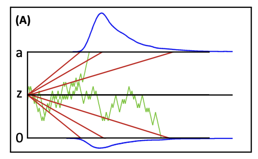
Figure 3.1: Graphical illuscation of simple sequential sampling model.
However, knowing the names and meanings of those parameters is not sufficient for R to generate data. You need to tell R (or any other programming software) the value of each parameter and how they should be used. Follow the steps below to plot the sampling path for a single trial.
3.2.1 Simulation: single trial (Step-by-step)
- Translate equation of DDM to R
Now, try to translate the equation below into R script. Don’t think too much, just type in what you see below (v refers to drift rate and sv refers to noise level):
Click to reveal example answer
# 1. Translate equation of DDM to R
evidence[timestep+1] <- evidence[timestep] + rnorm (mean = drift_rate, sd = noise, n = 1) # sample an evidence at each time point
Can you run the code? The error message might pop out because the computer does not not know the variable names (i.e., evidence? drift_rate? variance?) you mentioned above.
2. Determine parameter values
# 2. Determine parameter values
drift_rate <- 0.5  # 0 = noninformative stimulus; >0 = informative
threshold  <- 1.5     # separated boundary
noise   <- 0.02      # noise, SD of drift rate
Don’t forget to define starting point (z) and non-decision time (NDT).
# Determine parameter values for starting point and non-decision time
z <- threshold/2    # starting point. the middle of boundary if no bias.
NDT <-200           # time for non-decision related process, like motor execution
3. Determine number of time points (e.g., millisecond)
nsamples <- 10000 #Maximum sampling time point (ms)
dt       <- 0.001 # each time step is 1 ms (0.001second)
>
4. Create a variable to store output. Here, we are interested in evidence accumulation at each time point (i.e., total nsamples).
evidence <- rep(NA, 1, nsamples)
5. Initialize variable(s) and run the algorithm
 # Initialize variables. Initialization is important to make sure timestep starts from the first time point.
 # Moreover, we assume the evidence at the first time point starts from the starting point (i.e., E(t=1) = z).
  timestep <- 1
  evidence[1] = z;
6. Start accumulation with while loop:
# Start sampling until evidence reaches threshold
while (TRUE){
  # Sample evidence at each time point
  evidence[timestep+1] <- evidence[timestep] + rnorm(mean = drift_rate*dt, sd = noise, n = 1)

  # Check if evidence crosses any boundary (a or 0)
  if (evidence[timestep] >= threshold || evidence[timestep] < 0 || timestep == nsamples) {
    break
  }

  # Increment timestep
  timestep <- timestep + 1
}

# Model prediction about RT and choice
if (timestep >= nsamples) {
  # no RT and choice data if evidence does not reach the boundary before pre-determined time steps
  RT <- NA
  Choice <- NA
} else {
  RT <- timestep + NDT
  Choice <- which.min(c(abs(evidence[timestep]-0), abs(evidence[timestep]-threshold))) # choice = 2 if the evidence reached the upper boundary
}
Choice
## [1] 2RT## [1] 2689
7. visualize your simulation result (i.e., evidence accumulation in a trial)
#plot trajectories in stimulus-locked manner
plot(evidence[1:timestep],type = 'l',xlim = c(0,5000), xlab="RTs (ms)", ylim = c(0,threshold), ylab="Accumulated Evidence (unit)",
        main="Sampling path")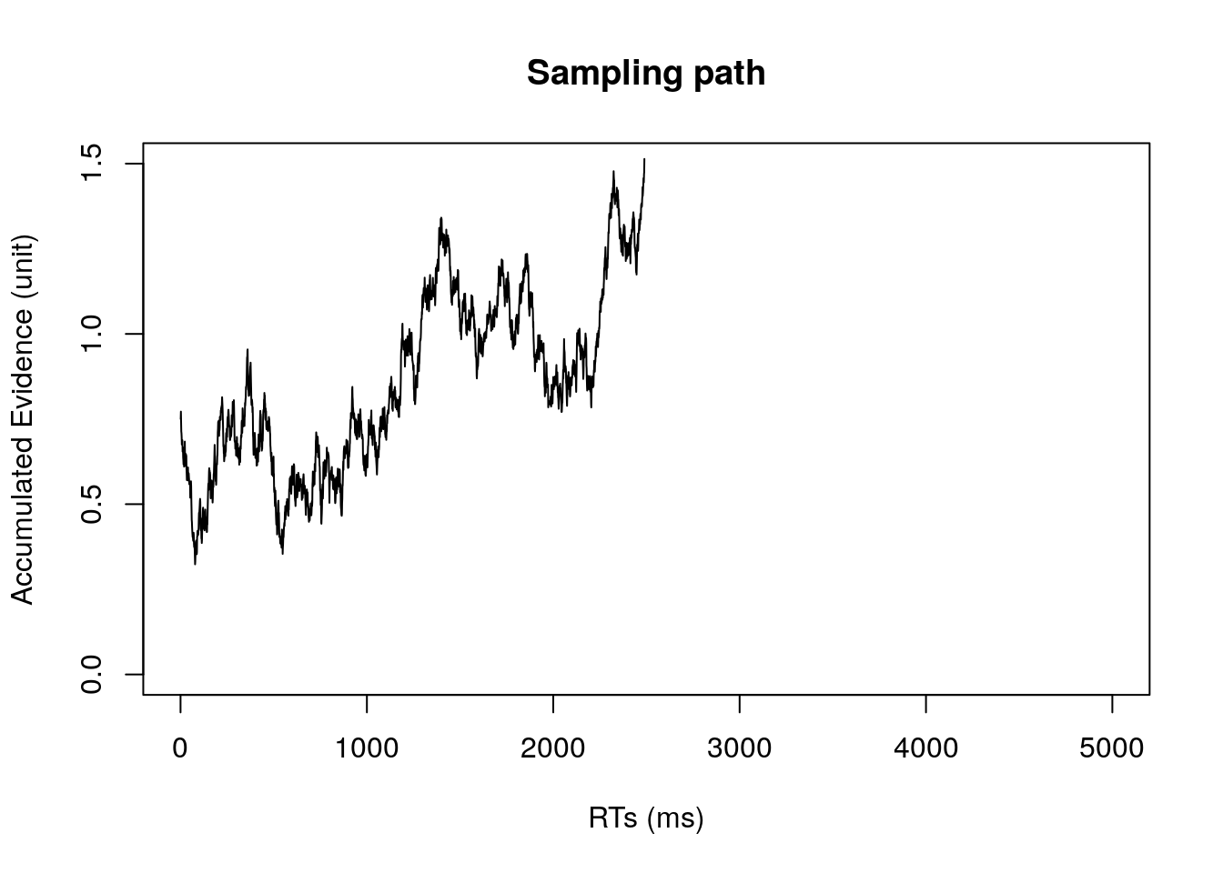
Task A:
Change noise value from 0.02 to 0. What do you observe?
8. Create a function that requires drift_rate and threshold as inputs and accumulated evidence as outputs.
# function of model1 (M1)
 model_1 <- function(drift_rate, threshold, noise, z, NDT){
   # Initialize variables. Initialization is important to make sure evidence and timestep start from rationale values.
   # Note: Unlike point 4-7, if you are not interested in the sampling path, evidence can be simply overwritten over time. Therefore, the size of each variable is not needed to be determined in advance.
   evidence <- z
   timestep <- 1
   nsamples <- 10000 #Maximum sampling time point (ms)
   dt       <- 0.001 # each time step is 1 ms (0.001second)


   # Start sampling until evidence reaches threshold
   while (TRUE){
     # Sample evidence at each time point
     evidence <- evidence + rnorm(mean = drift_rate*dt, sd = noise, n = 1)

     # Check if evidence crosses any boundary (a or 0)
     if (evidence >= threshold || evidence < 0 || timestep == nsamples) {
       break
     }

     # Increment timestep
     timestep <- timestep + 1
   }

   # Model prediction about RT and choice
   if (timestep >= nsamples) {
     # no RT and choice data if evidence does not reach the boundary before pre-determined time steps
     RT <- NA
     Choice <- NA
   } else {
     RT <- timestep + NDT
     Choice <- which.min(c(abs(evidence-0), abs(evidence-threshold))) # choice = 2 if the evidence reached the upper boundary
   }

  return(list(Choice, RT))
}
### Simulation: multipl trials
# with the function, we can simulate data for multiple trials (e.g., 1000 trials)
# Determine parameter values
drift_rate <- 0.5  # 0 = noninformative stimulus; >0 = informative
threshold  <- 1.5    # separated boundary
noise   <- 0.02  # noise, variance of drift rate
z <- threshold/2    # starting point. the middle of boundary if no bias.
NDT <-200           # time for non-decision related process, like motor execution

# Determine number of trials
n_trial <- 1000

#Pre-allocate the size for output of interest
response_times <- rep(NA, 1, n_trial)
ChooseA <- rep(NA, 1, n_trial)

# run the main script
for (k_trial in 1:n_trial){
  results <- model_1(drift_rate = drift_rate,
                     threshold = threshold,
                     noise = noise,
                     z = z, NDT = NDT)
  ChooseA[k_trial] <-results[[1]]
  response_times[k_trial] <-results[[2]]
}
finally, you can plot the RT distribution of your simulation.
# draw RT distribution as histogram
hist(response_times[ChooseA==2],xlab="RT (ms)", xlim=c(0, nsamples), breaks="FD", col = alpha("red", 0.3), main="RT distribution (for correct/incorrect choices)")
hist(response_times[ChooseA==1],xlab="RT (ms)", xlim=c(0, nsamples), , breaks="FD", col = alpha("black", 0.3), add=T)

# Add legend for both histogram and mean lines
legend("topright", legend = c("Correct", "Inocorrect"), fill = c(alpha("red", 0.5), alpha("black", 0.3), "red", "black"), cex = 0.8)
Task B:
Run model_1 multiple times with noise = 0 and summarize the RT distribution. What do you observe when you compare the results with noise of 0.02?
3.3 Model2: Drfit-diffusion model (with condition-dependent drift rates)
3.3.1 Create a Function
model_2 <- function(drift_list, threshold, noise, z, NDT, cond){
  # suppose cond is a list of 1 and 2 for two conditions.

  # Initialize variables.
  evidence <- z
  timestep <- 1
  nsamples <- 10000 #Maximum sampling time point (ms)
  dt       <- 0.001 # each time step is 1 ms (0.001second)

  drift_rate <- drift_list[cond]

  # Start sampling until evidence reaches threshold
  while (TRUE){
    # Sample evidence at each time point
    evidence <- evidence + rnorm(mean = drift_rate*dt, sd = noise, n = 1)

     # Check if evidence crosses any boundary (a or 0)
     if (evidence >= threshold || evidence < 0 || timestep == nsamples) {
       break
     }

     # Increment timestep
     timestep <- timestep + 1
   }

   # Model prediction about RT and choice
   if (timestep >= nsamples) {
     # no RT and choice data if evidence does not reach the boundary before pre-determined time steps
     RT <- NA
     Choice <- NA
   } else {
     RT <- timestep + NDT
     Choice <- which.min(c(abs(evidence-0), abs(evidence-threshold))) # choice = 2 if the evidence reached the upper boundary
   }

  return(list(cond, Choice, RT))
}
3.3.2 Simulation
# with the function, we can simulate data for multiple trials (e.g., 1000 trials)
# Determine parameter values
m2.drift_list<- c(0.5,0.9)  # 0 = noninformative stimulus; >0 = informative
m2.threshold  <- 1.5    # separated boundary
m2.noise   <- 0.02  # noise, variance of drift rate
m2.z <- m2.threshold/2    # starting point. the middle of boundary if no bias.
m2.NDT <-200           # time for non-decision related process, like motor execution

# Determine number of trials
m2.n_trial <- 1000
m2.cond <- sample(c(1,2), 1000, replace = TRUE)

#Pre-allocate the size for output of interest
m2.data <-  matrix(NA, m2.n_trial, 3)

# run the main script
for (k_trial in 1:m2.n_trial){

  results <- model_2(m2.drift_list,
                     m2.threshold,
                     m2.noise,
                     m2.z,
                     m2.NDT,
                     m2.cond[k_trial])

    # Save results in m2.data matrix
  results
  m2.data[k_trial, 1] <- results[[1]]
  m2.data[k_trial, 2] <- results[[2]]
  m2.data[k_trial, 3] <- results[[3]]
}
3.3.3 Visualization
We can quickly take a look overall RT distribution by calling hist to plot the histogram of RT.
# RTs distribution regardless of conditions
hist(m2.data[,3],xlab="RT (ms)", xlim=c(0,4000), breaks="FD", main="RT distribution of M2")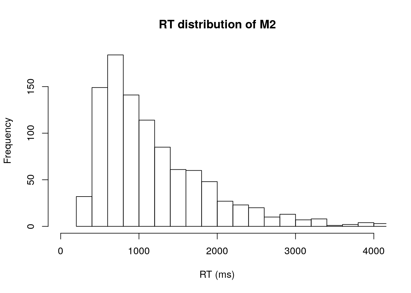
Alternatively, we can separately plot the RT for different conditions.
# RTs of condition1
ID.condition1 = m2.data[,1] == 1
hist(m2.data[ID.condition1,3],xlab="RT (ms)", xlim=c(0,4000), ylim=c(0,200), breaks="FD", main="RT distribution (for different drift rates)", col = alpha("blue", 0.5))


# RTs of condition2
ID.condition2 = m2.data[,1] == 2
hist(m2.data[ID.condition2,3],xlab="RT (ms)", xlim=c(0,4000), breaks="FD", col = alpha("green", 0.3), add=T)

# Add legend for both histogram and mean lines
legend("topright", legend = c("Condition1", "Condition2"), fill = c(alpha("blue", 0.5), alpha("green", 0.3), "blue", "green"), cex = 0.8)
ID.condition1 = m2.data[,1] == 1
ID.condition2 = m2.data[,1] == 2
# Calculate mean RT and accuracy for each condition
mean_RT_condition1 <- mean(m2.data[ID.condition1, 3], na.rm = TRUE)
mean_RT_condition2 <- mean(m2.data[ID.condition2, 3], na.rm = TRUE)
mean_ACC_condition1 <- mean(m2.data[ID.condition1, 2] ==2, na.rm = TRUE)
mean_ACC_condition2 <- mean(m2.data[ID.condition2, 2] ==2, na.rm = TRUE)
# Store aggregate data
data_matrix<- matrix(data = NA, nrow = 2, ncol = 3)
data_matrix[1, ]<-c(m2.drift_list[1], mean_RT_condition1, mean_ACC_condition1)
data_matrix[2, ]<-c(m2.drift_list[2], mean_RT_condition2, mean_ACC_condition2)
# Add row and column names
rownames(data_matrix) <- c("Condition1", "Condition2")
colnames(data_matrix) <- c("Drift rate", "Mean RT", "Mean Accuracy")
print(data_matrix)## Drift rate Mean RT Mean Accuracy
## Condition1 0.5 1376.458 0.8681542
## Condition2 0.9 1058.091 0.97633143.4 Model3: Drfit-diffusion model (with condition-dependent threshold)
3.4.1 Create a Function
Now, let’s create our third model by modifying model_2. Instead of having condition-dependent drift rates, model_3 has condition-dependent threshold (and starting point.
model_3 <- function(drift_rate, threshold_list, noise, z_list, NDT, cond){
  # suppose cond is a list of 1 and 2 for two conditions.

  # determine the condition-dependent parameters
  threshold <- threshold_list[cond]
  z <- z_list[cond]

  # Initialize variables
  evidence <- z
  timestep <- 1
  nsamples <- 10000 #Maximum sampling time point (ms)
  dt       <- 0.001 # each time step is 1 ms (0.001second)


  # Start sampling until evidence reaches threshold
  while (TRUE){
    # Sample evidence at each time point
    evidence <- evidence + rnorm(mean = drift_rate*dt, sd = noise, n = 1)

     # Check if evidence crosses any boundary (a or 0)
     if (evidence >= threshold || evidence < 0 || timestep == nsamples) {
       break
     }

     # Increment timestep
     timestep <- timestep + 1
   }

   # Model prediction about RT and choice
   if (timestep >= nsamples) {
     # no RT and choice data if evidence does not reach the boundary before pre-determined time steps
     RT <- NA
     Choice <- NA
   } else {
     RT <- timestep + NDT
     Choice <- which.min(c(abs(evidence-0), abs(evidence-threshold))) # choice = 2 if the evidence reached the upper boundary
   }

  return(list(cond, Choice, RT))
}
3.4.2 Simulation
# with the function, we can simulate data for multiple trials (e.g., 1000 trials)
# Determine parameter values
m3.drift_rate<- 0.5  # 0 = noninformative stimulus; >0 = informative
m3.threshold_list  <- c(1.2, 1.5)    # separated boundary
m3.noise   <- 0.02  # noise, variance of drift rate
m3.z_list <- m3.threshold_list/2    # starting point. the middle of boundary if no bias.
m3.NDT <-200           # time for non-decision related process, like motor execution

# Determine number of trials
m3.n_trial <- 1000
m3.cond <- sample(c(1,2), 1000, replace = TRUE)

#Pre-allocate the size for output of interest
m3.data <-  matrix(NA, m3.n_trial, 3)

# run the main script
for (k_trial in 1:m3.n_trial){

  results <- model_3(m3.drift_rate,
                     m3.threshold_list,
                     m3.noise,
                     m3.z_list,
                     m3.NDT,
                     m3.cond[k_trial])

    # Save results in m2.data matrix
  results
  m3.data[k_trial, 1] <- results[[1]]
  m3.data[k_trial, 2] <- results[[2]]
  m3.data[k_trial, 3] <- results[[3]]
}
3.4.3 Visualization
We can quickly take a look overall RT distribution by calling hist
# RTs distribution regardless of condition
hist(m3.data[,3],xlab="RT (ms)", xlim=c(0,5000), breaks="FD", main="RT distribution of M3")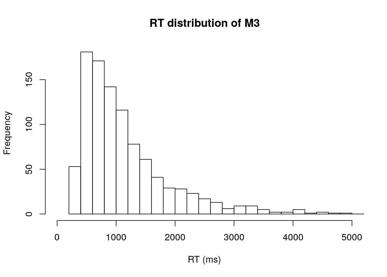
Alternatively, we can separately plot the RT for different conditions.
# RTs of condition1
ID.condition1 = m3.data[,1] == 1
hist(m3.data[ID.condition1,3],xlab="RT (ms)", xlim=c(0,5000), ylim=c(0,200), breaks="FD", main="RT distribution (for different drift rates)", col = alpha("blue", 0.5))


# RTs of condition2
ID.condition2 = m3.data[,1] == 2
hist(m3.data[ID.condition2,3],xlab="RT (ms)", xlim=c(0,5000), breaks="FD", col = alpha("green", 0.3), add=T)

# Add legend for both histogram and mean lines
legend("topright", legend = c("Condition1", "Condition2"), fill = c(alpha("blue", 0.5), alpha("green", 0.3), "blue", "green"), cex = 0.8)
ID.condition1 = m3.data[,1] == 1
ID.condition2 = m3.data[,1] == 2
# Calculate mean RT and accuracy for each condition
mean_RT_condition1 <- mean(m3.data[ID.condition1, 3], na.rm = TRUE)
mean_RT_condition2 <- mean(m3.data[ID.condition2, 3], na.rm = TRUE)
mean_ACC_condition1 <- mean(m3.data[ID.condition1, 2] ==2, na.rm = TRUE)
mean_ACC_condition2 <- mean(m3.data[ID.condition2, 2] ==2, na.rm = TRUE)
# Store aggregate data
data_matrix<- matrix(data = NA, nrow = 2, ncol = 3)
data_matrix[1, ]<-c(m3.threshold_list[1], mean_RT_condition1, mean_ACC_condition1)
data_matrix[2, ]<-c(m3.threshold_list[2], mean_RT_condition2, mean_ACC_condition2)
# Add row and column names
rownames(data_matrix) <- c("Condition1", "Condition2")
colnames(data_matrix) <- c("Threshold", "Mean RT", "Mean Accuracy")
print(data_matrix)## Threshold Mean RT Mean Accuracy
## Condition1 1.2 981.464 0.8125000
## Condition2 1.5 1362.129 0.8855932