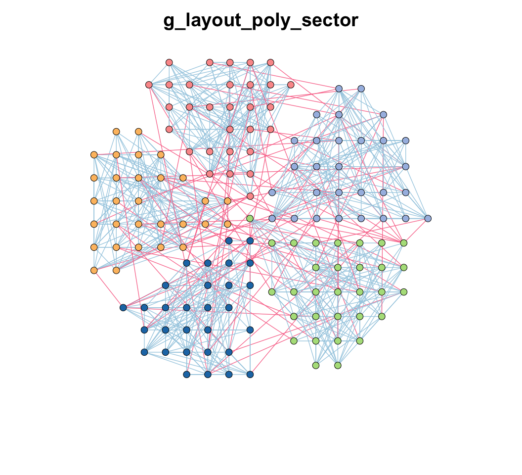
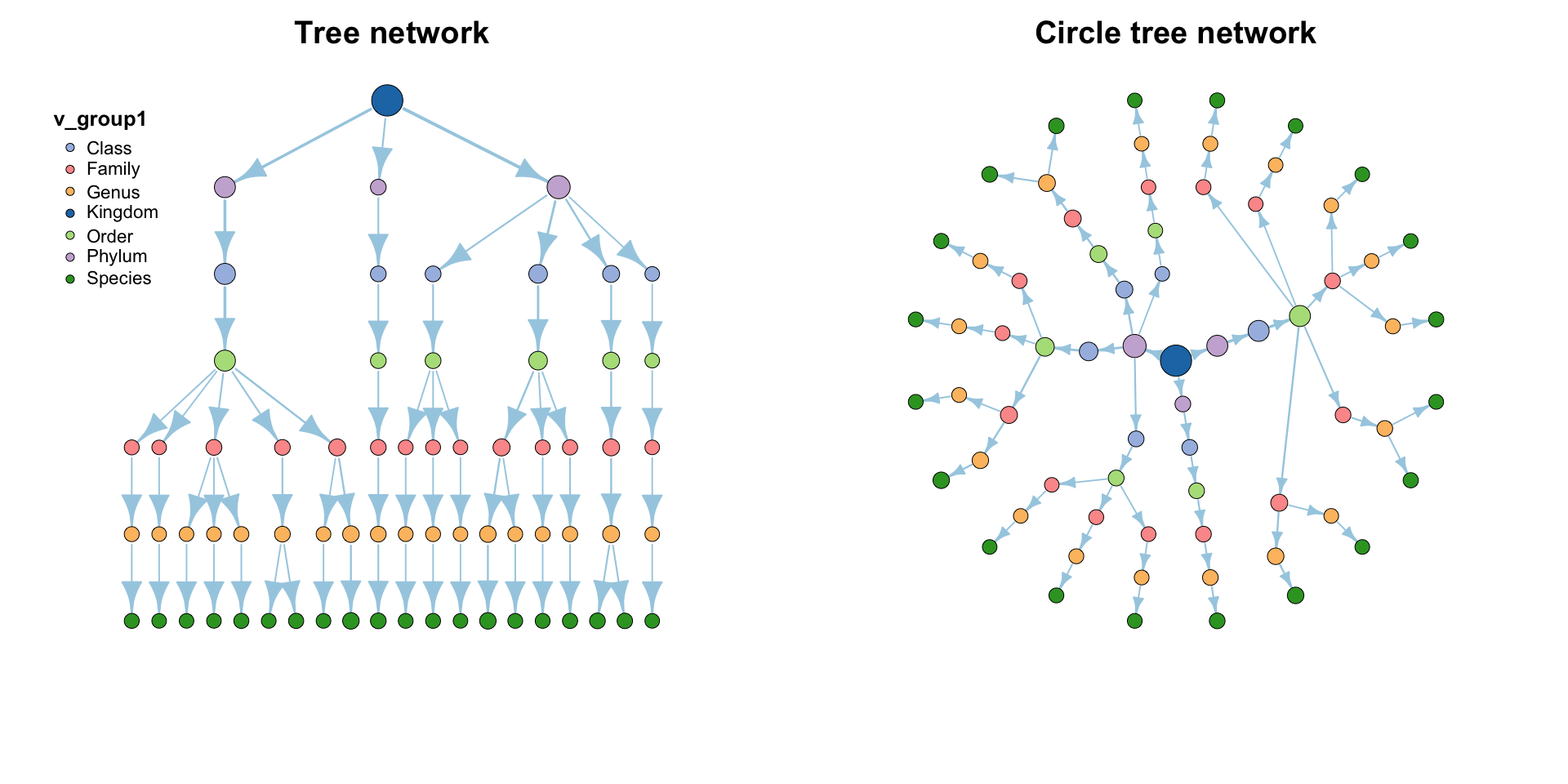
data("multi_test", package = "MetaNet")
data("c_net", package = "MetaNet")
# build a multi-network
<- multi_net_build(list(Microbiome = micro, Metabolome = metab, Transcriptome = transc))
multi1 # v_group is default, three different table
plot(multi1)
# set vertex_class
<- c_net_set(multi1, micro_g, metab_g, transc_g, vertex_class = c("Phylum", "kingdom", "type"))
multi1_with_anno # set vertex_size
<- c_net_set(multi1_with_anno,
multi1_with_anno data.frame("Abundance1" = colSums(micro)),
data.frame("Abundance2" = colSums(metab)),
data.frame("Abundance3" = colSums(transc)),
vertex_size = paste0("Abundance", 1:3)
)
plot(multi1_with_anno)
4 Visualization
MetaNet
supports basic R plot and provides some interfaces for other software (Gephi
, Cytoscape
, ggplot2
, networkD3
) to visualize, while there are also a lot of layout methods for better display.
4.1 Basic plot
Set attributes
As we mentioned before, there are some internal attributes have been set when building network, which are related to the network visualization (Table 3.1). So we can use c_net_set()
to custom these attributes fitting to our research needs.
Give the network various annotate tables and determine which columns use to set, we can give the columns name (one or more) to vertex_group
, vertex_class
, vertex_size
, edge_type
, edge_class
, edge_width
.
And the colors, linetypes, shapes and legends will be assigned automatically, just use plot()
to get the basic metanet figure. For more details to customize the plot, refer to Table 4.1.
Plot setting
If you want to custom the network plot flexibility, use the c_net_plot()
which contains many flexible arguments. The arguments of c_net_plot()
are listed below:
c_net_plot()
arguments.
Arguments | Description |
---|---|
coors | 
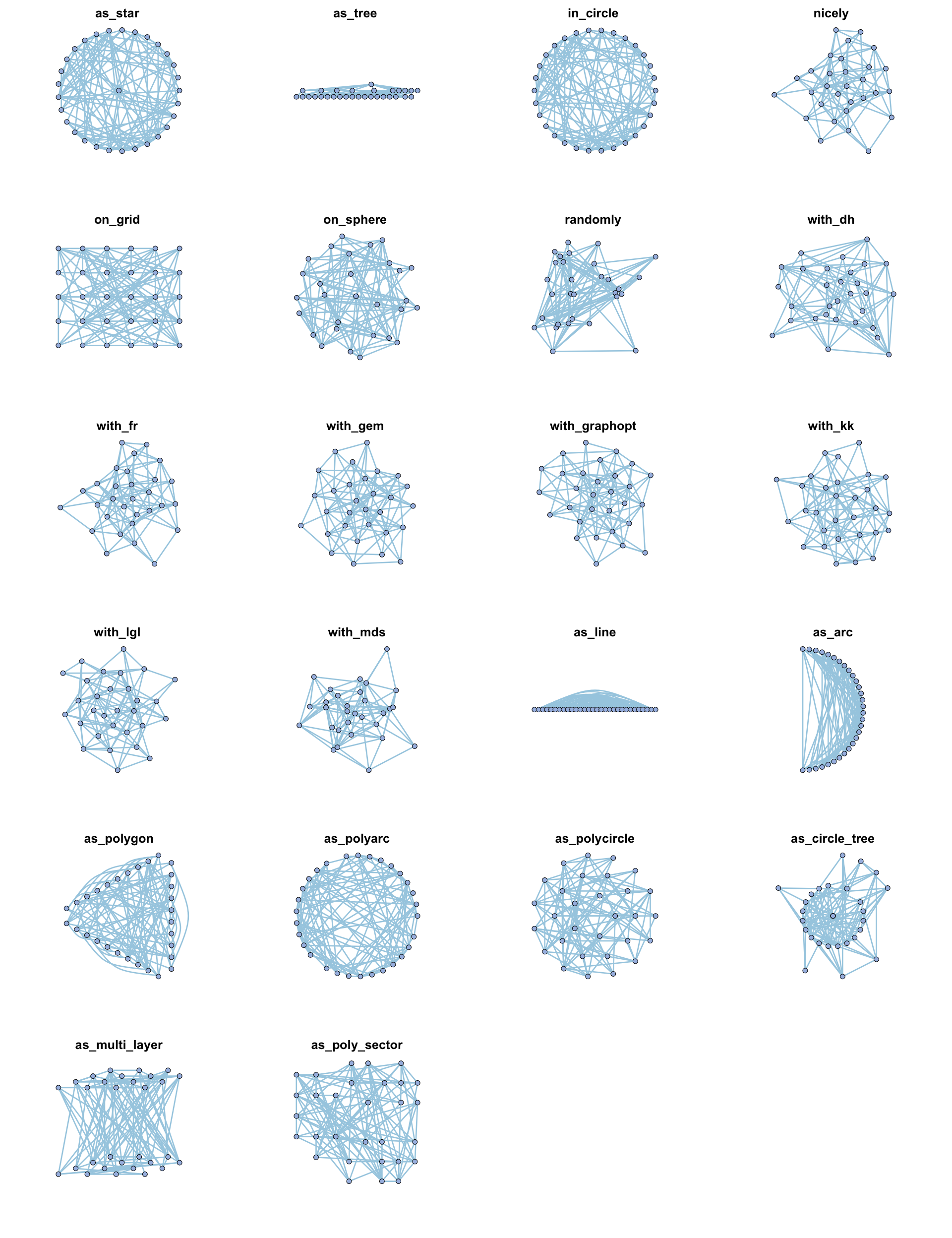
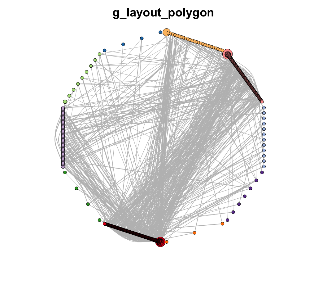
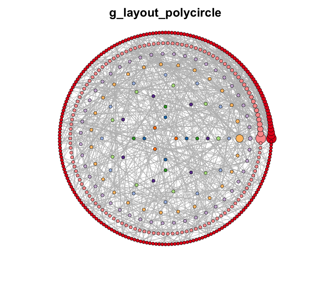
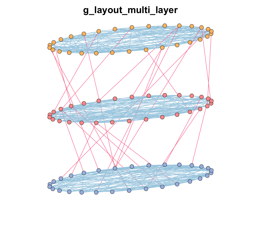
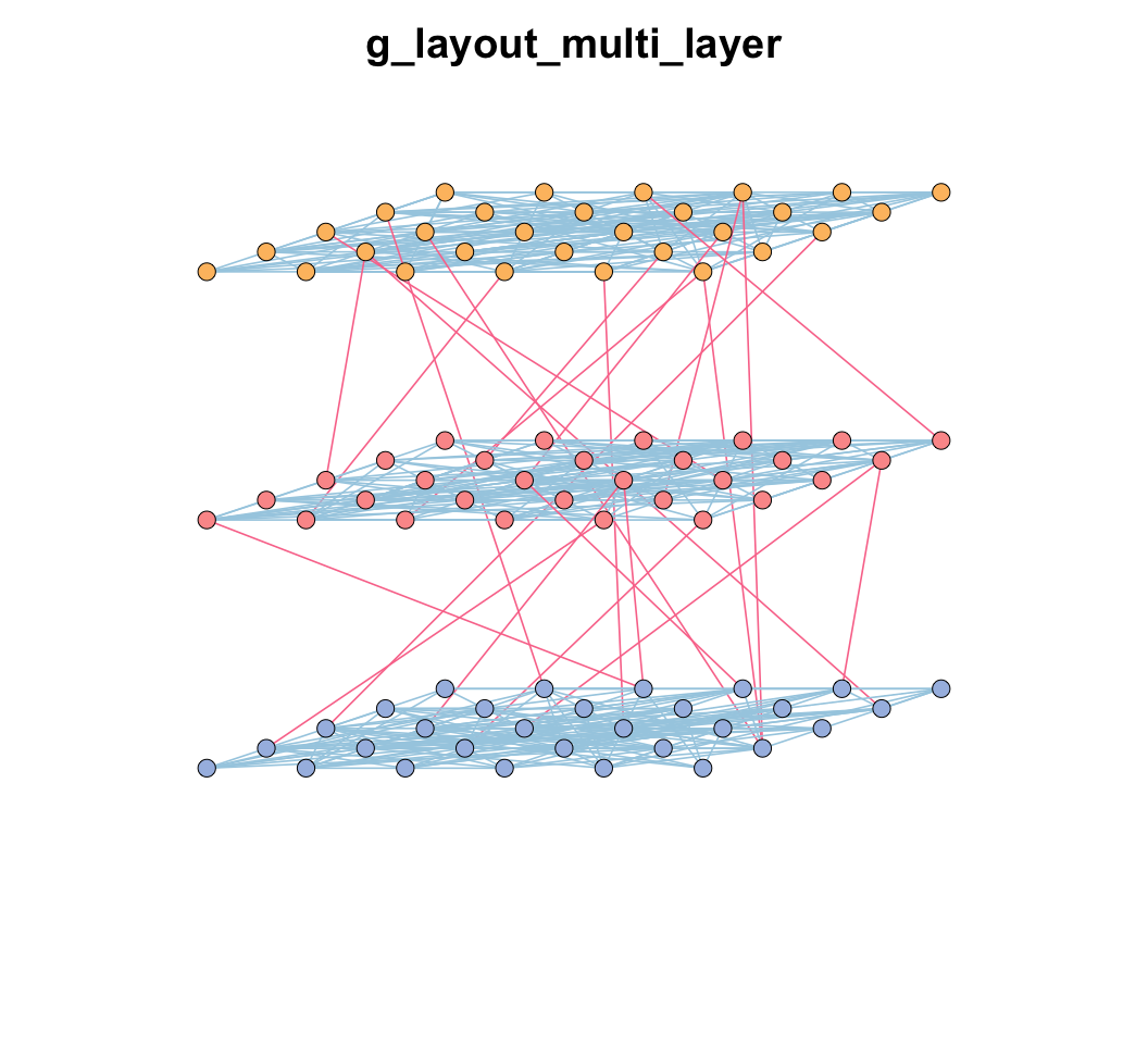
1. cooridnates dataframe, 2. layout function (e.g. as_star(), as_tree(), in_circle(), nicely()... see help(c_net_lay)) |
vertex.color | color of nodes, receive vector (1. length same to number of nodes; 2. length same to numbers of v_class; 3. named verctor like c(A="red",B="blue")) |
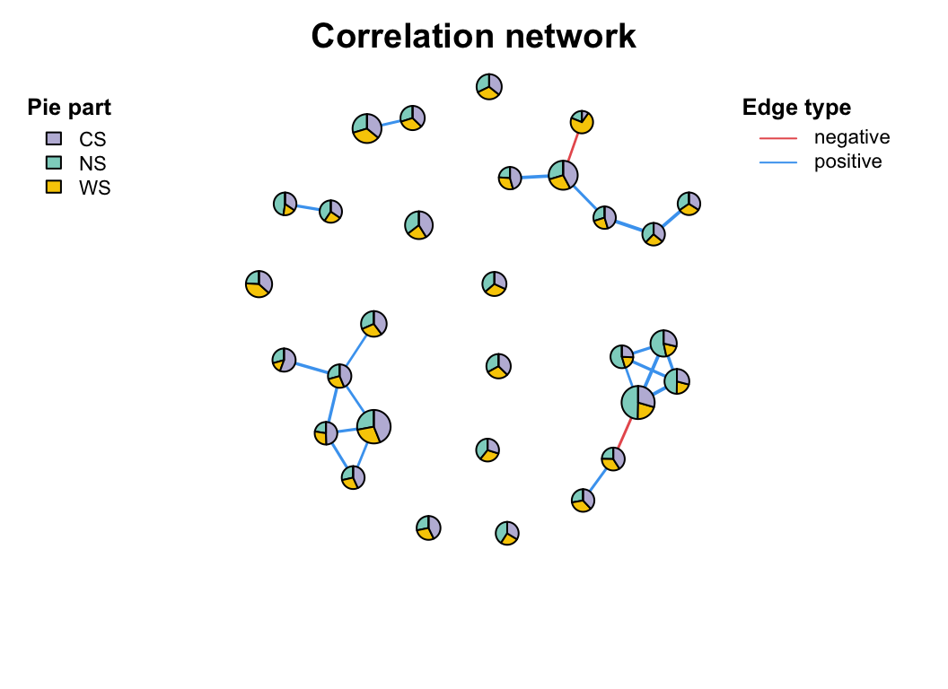
vertex. shape | shape of nodes, receive vector (1. length same to number of nodes; 2. length same to numbers of v_group; 3. named verctor like c(v_group1="circle",B="square"))shape list: none, circle, square, csquare, rectangle, crectangle, vrectangle, pie, raster, or sphere |
vertex.size | size of nodes, receive numerical vector (length same to number of nodes)please use mmscale to control vertex.size, don't be too large. |
vertex_size_range | the vertex size range, e.g. c(1,10) |
labels_num | show how many labels,>1 indicates number, |
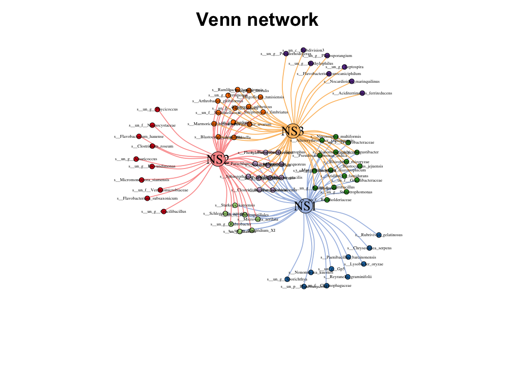
vertex.label | the label of nodes, NA indicates no label |
vertex.label.family | label font family |
vertex.label.font | label font, 1 plain, 2 bold, 3 italic, 4 bold italic, 5 symbol |
vertex.label.cex | label size |
vertex.label.dist | distance from label to nodes |
vertex.label.color | The color of the labels, The default value is black. |
vertex.label.degree | 0:right, pi: left, pi/2:below, -pi/2:above |
vertex.frame.color | color of nodes frame |
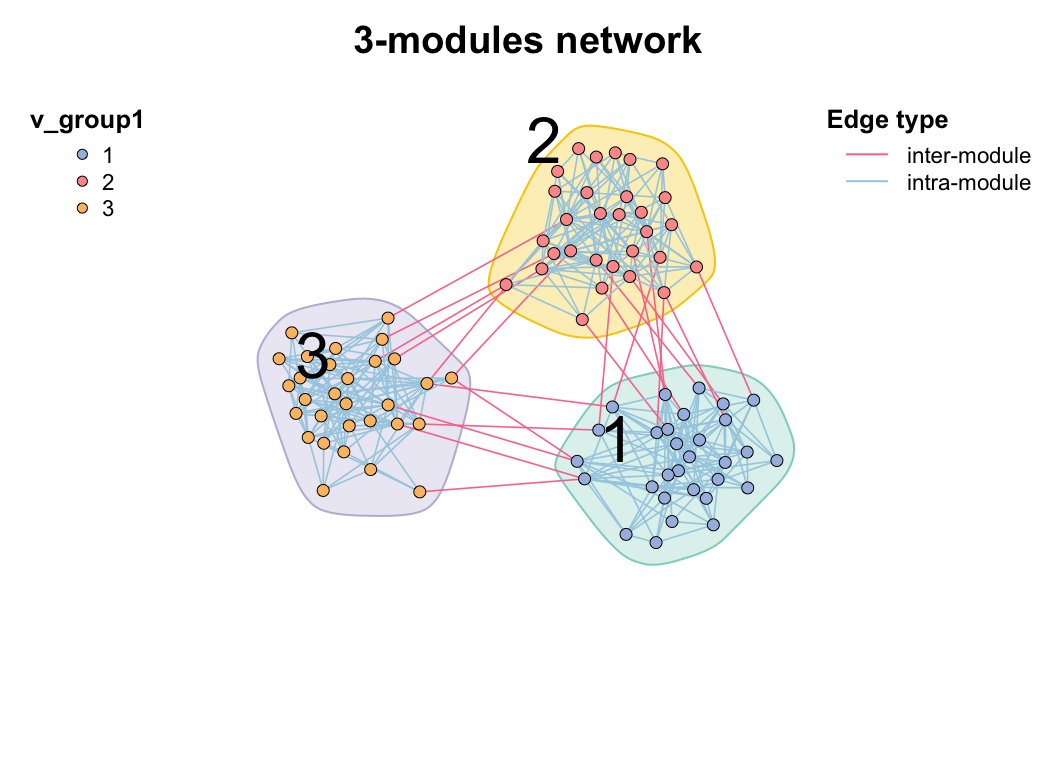
plot_module | use module as the v_class |
mark_module | logical, mark the modules? |
mark_color | mark color |
mark_alpha | mark fill alpha, default 0.3 |
module_label | show module label? |
module_label_cex | module label cex |
module_label_color | module label color |
module_label_just | module label just, default c(0.5,0.5) |
edge.color | color of edges, receive vector (1. length same to number of edges; 2. length same to numbers of e_type; 3. named verctor like c(A="red",B="blue")) |
edge.width | width of edge, receive numerical vector (length same to number of edges)please use mmscale to control vertex.size, don't be too large. |
edge_width_range | the edge width range, e.g. c(1,10) |
edge.lty | linetype of edge, receive vector (1. length same to number of edges; 2. length same to numbers of e_class; 3. named verctor like c(A="red",B="blue")) |
edge.arrow.size | arrow size for directed network |
edge.arrow.width | arrow width for directed network |
arrow.mode | arrow mode, 0 no arrow, 1 back, 2 forward, 3 both |
edge.label | the label of edges, NA indicates no label |
edge.label.family | label font family |
edge.label.font | label font, 1 plain, 2 bold, 3 italic, 4 bold italic, 5 symbol |
edge.label.cex | label size |
edge.label.x | label x-axis |
edge.label.y | label y-axis |
edge.label.color | label color |
edge.curved | The curvature of the body, on a scale of 0-1, FALSE means 0, TRUE means 0.5 |
legend | show any legend? FALSE means close all legends |
legend_cex | character expansion factor relative to current par('cex'), default: 1 |
legend_position | legend_position, default: c(left_leg_x=-1.9,left_leg_y=1,right_leg_x=1.2,right_leg_y=1) |
legend_number | add numbers in legend? (v_class number, e_type number...) |
lty_legend, lty_legend_title, lty_legend_order | show lty_legend? and the title, the oreder of legend receives a vector |
size_legend, size_legend_tiltle | show size_legend? and the title |
edge_legend, edge_legend_title, edge_legend_order | show edge_legend? and the title, the order of legend receives a vector |
width_legend, width_legend_title | show width_legend? and the title |
color_legend, color_legend_order | show col_legend? and the title, the order of legend receives a vector |
group_legend_title, group_legend_order | the title of group, the order of legend receives a vector |
margin | margin, a vector whose length =4 |
rescale | scale the coors to [-1,1], default F |
asp | y/x ratio |
frame | if T, add frame |
main | the main title of graph |
sub | subtitle |
xlab | x-axis label |
ylab | y-axis label |
seed | random seed, default:1234, make sure each plot is the same |
params_list | a list of parameters, e.g. list(edge_legend = TRUE, lty_legend = FALSE), when the parameter is duplicated, the format argument will be used rather than the argument in params_list |
For example, we can use c_net_plot()
to plot the network with annotation and set the color, size, width, legend, etc.
c_net_plot(multi1_with_anno,
labels_num = 5, vertex.color = get_cols(11, "col1"), vertex_size_range = c(3, 10), vertex.label.color = "red",
edge_width_range = c(0.5, 3), edge.color = c("orange", "green4"), edge.curved = 0.2,
legend = T, legend_number = T, group_legend_order = c("Microbiome", "Metabolome", "Transcriptome"),
group_legend_title = c("Phylum", "Metabolome", "Transcriptome"),
edge_legend_title = "Correlation", edge_legend_order = c("positive", "negative"),
size_legend = T, size_legend_title = "Abundance",
width_legend = T, width_legend_title = "abs(r)",
lty_legend = T, lty_legend_title = "Omics relationship"
)
params_list
is a special argument in c_net_plot()
, it is a list contains parameters, it is very convenient to use it to plot a series of network with same attributes.
<- setNames(get_cols(9, "col1"), unique(V(multi1_with_anno)$v_class))
node_colors
<- list(
params_list coors=c_net_layout(multi1_with_anno),
labels_num = 5,
vertex.color = node_colors, vertex_size_range = c(3, 10), vertex.label.color = "red",
edge_width_range = c(0.5, 3), edge.color = c("orange", "green4"), edge.curved = 0.2,
legend = T, legend_number = T, group_legend_order = c("Microbiome", "Metabolome", "Transcriptome"),
group_legend_title = c("Phylum", "Metabolome", "Transcriptome"),
edge_legend_title = "Correlation", edge_legend_order = c("positive", "negative"),
size_legend = T, size_legend_title = "Abundance",
width_legend = T, width_legend_title = "abs(r)",
lty_legend = T, lty_legend_title = "Omics relationship"
)
c_net_plot(multi1_with_anno, params_list = params_list)
# build another multi-network
<- c_net_filter(multi1_with_anno, v_group %in% c("Microbiome", "Metabolome")) %>%
multi1_with_anno2 c_net_filter(., e_class == "intra", mode = "e")
c_net_plot(multi1_with_anno2, params_list = params_list)
4.2 Layout
Layout is an important part of network visualization, a good layout will present information clearly.
So, in MetaNet
, we always use a coors
object to store the coordinates of a layout.
The coors
is a three-columns data.frame contains “name”, “X”, “Y”. attributes(coors)$curved
is a three-columns data.frame contains “from”, “to”, “curved” or NULL.
Basic layout
Use c_net_layout()
to get coordinates with specific layout methods.
c_net_layout(co_net2, method = in_circle()) -> coors
c_net_plot(co_net2, coors)
The method can be one of
as_line()
,as_arc()
,as_polygon()
,as_polyarc()
,as_polycircle()
,as_circle_tree()
,as_multi_layer()
,as_poly_sector()
.layouts in igraph:
in_circle()
,nicely()
,on_grid()
,on_sphere()
,randomly()
,with_dh()
,with_fr()
,with_gem()
,with_graphopt()
,with_kk()
,with_lgl()
,with_mds()
, seeigraph::layout_()
.layouts in ggraph: a character, “auto”, “backbone”, “centrality”, “circlepack”, “dendrogram”, “eigen”, “focus”, “hive”, “igraph”, “linear”, “manual”, “matrix”, “partition”, “pmds”, “stress”, “treemap”, “unrooted”. see
ggraph::create_layout()
.
Code
<- erdos.renyi.game(30, 0.25)
go # get a metanet
<- c_net_update(go)
go
<- list(
layout_methods as_star(), as_tree(), in_circle(), nicely(),
on_grid(), on_sphere(), randomly(), with_dh(),
with_fr(), with_gem(), with_graphopt(), with_kk(),
with_lgl(), with_mds(), as_line(), as_arc(),
as_polygon(), as_polyarc(), as_polycircle(3), as_circle_tree(),
as_multi_layer(2), as_poly_sector()
)names(layout_methods) <- c(
"as_star ", "as_tree ", "in_circle ", "nicely ",
"on_grid ", "on_sphere ", "randomly ", "with_dh ",
"with_fr ", "with_gem ", "with_graphopt ", "with_kk ",
"with_lgl ", "with_mds", "as_line", "as_arc",
"as_polygon", "as_polyarc", "as_polycircle", "as_circle_tree",
"as_multi_layer", "as_poly_sector"
)
par(mfrow = c(6, 4))
for (i in names(layout_methods)) {
plot(go, layout_methods[[i]], legend = F, main = i, labels_num = 0)
}
And for each method, you can add some arguments in it:
# get a metanet
<- erdos.renyi.game(30, 0.25)
go <- c_net_update(go)
go
plot(go, coors = with_fr())
plot(go, coors = with_fr(niter = 99, grid = "nogrid"))
The as_polygon()
is interesting: it can draw a network in a polygon shape, and you can change the edge numbers of the polygon.
Transform layout
Using transform_comors
can transform layouts, including zooming in and out, X/Y ratio, rotation angle, mirroring, pseudo 3D effects, etc.:
Group layout
Beside the c_net_layout()
, we provide an advanced layout method for a network with group variable: g_layout()
. It is easy to use g_layout()
to control each group position and layout of each group.
g_layout()
is a very useful function to layout a network with group variable when we have a multi-omics network (Chapter 7) or module network (Section 5.4).
- First, assign a group variable.
- Give a
layout1
for group position, one of 1.a dataframe or matrix: rowname is group, two columns are X and Y 2.function: layout method forc_net_layout()
default: in_circle() - Adjust the
zoom1
oflayout1
. - Give a
layout2
(layout method forc_net_layout()
) for each group layout, or use a list contains functions match each group. - Adjust the
zoom2
oflayout2
, you can use a vector to adjust each group zoom. - use
show_big_layout = T
to see thelayout1
distribution.
par(mfrow = c(2, 1))
# set circle layout for each group
g_layout(multi1_with_anno,
group = "v_group", layout1 = in_circle(),
zoom1 = 10, layout2 = in_circle(), zoom2 = 5
-> g_coors
) plot(multi1_with_anno, coors = g_coors)
# set different layout for each group
g_layout(multi1_with_anno,
group = "v_group", layout1 = in_circle(), zoom1 = 10,
layout2 = list(in_circle(), with_fr(), as_polygon()), zoom2 = 3:5
-> g_coors
) plot(multi1_with_anno, coors = g_coors)
As layout1
also receive a matrix or data.frame, so we can use the group skeleton of network to adjust the layout1
.
data("c_net", package = "MetaNet")
g_layout(co_net,
group = "v_class", layout1 = in_circle(), zoom1 = 10,
layout2 = in_circle(), zoom2 = c(1, 5, 2, 1, 3, 7)
-> g_coors
) plot(co_net, coors = g_coors)
# firstly get the skeleton plot
get_group_skeleton(co_net, "v_class") %>% clean_igraph() -> s_net
# then use tkplot to do manual adjustment.
<- igraph::tkplot(s_net)
x # Here: Move nodes within the tkplot window to a layout you like!
<- igraph::tkplot.getcoords(x)
da # close the window
::tkplot.close(x)
igraph# pass the `da` to layout1
g_layout(co_net,
group = "v_class", layout1 = da, zoom1 = 20,
layout2 = in_circle(), zoom2 = c(1, 4, 2, 1, 3, 5)
-> g_coors
) plot(co_net, coors = g_coors)
g_layout()
provides a high degree of customization, you can adjust the layout according to different needs.
Besides, there are also some good default group layout methods: - g_layout_circlepack()
- g_layout_treemap()
- g_layout_backbone()
- g_layout_stress()
- g_layout_polyarc()
- g_layout_polygon()
- g_layout_polycircle()
- g_layout_multi_layer()
- g_layout_poly_sector()
Code
E(co_net)$color <- rep("grey", length(E(co_net)))
plot(co_net,
coors = g_layout_circlepack(co_net, group = "v_class"),
legend = F, labels_num = 0, main = "g_layout_circlepack"
)
plot(co_net,
coors = g_layout_treemap(co_net, group = "v_class"),
legend = F, labels_num = 0, main = "g_layout_treemap"
)
plot(co_net,
coors = g_layout_backbone(co_net, group = "v_class"),
legend = F, labels_num = 0, main = "g_layout_backbone"
)
plot(co_net,
coors = g_layout_stress(co_net, group = "v_class"),
legend = F, labels_num = 0, main = "g_layout_stress"
)
plot(co_net,
coors = g_layout_polyarc(co_net, group = "v_class"),
legend = F, labels_num = 0, main = "g_layout_polyarc"
)
plot(co_net,
coors = g_layout_polygon(co_net, group = "v_class"),
legend = F, labels_num = 0, main = "g_layout_polygon"
)
plot(co_net,
coors = g_layout_polycircle(co_net, group = "v_class"),
legend = F, labels_num = 0, main = "g_layout_polycircle"
)
<- module_net(3)
g1 plot(g1,
coors = g_layout_multi_layer(g1, group = "v_class"),
legend = F, labels_num = 0, main = "g_layout_multi_layer"
)
plot(g1,
coors = g_layout_multi_layer(g1, group = "v_class", layout = on_grid()),
legend = F, labels_num = 0, main = "g_layout_multi_layer"
)
<- module_net(5)
g2 plot(g2,
coors = g_layout_poly_sector(g2, group = "v_class"),
legend = F, labels_num = 0, main = "g_layout_poly_sector"
)
spatstat
layout
You can also use spatstat
to construct any polygon, and then randomly or uniformly sample the interior or edges of the polygon to generate a layout:
if(!require("spatstat"))install.packages("spatstat")
<- c(0, 2, 2, 0)
poly_x <- c(0, 0, 1, 1)
poly_y <- spatstat.geom::owin(poly = list(x = poly_x, y = poly_y))
win_poly plot(win_poly)
<- spatstat_layout(co_net, win_poly, type = "random", mode = "surface")
coors1 plot(co_net, coors = coors1)
<- spatstat_layout(co_net, win_poly, type = "regular", mode = "surface",order_by="v_class")
coors1 plot(co_net, coors = coors1)
<- spatstat_layout(co_net2, win_poly, type = "random", mode = "boundary")
coors2 plot(co_net2, coors = coors2)
Try a ⭐️:
library(spatstat.geom)
<- function(r_outer = 1, r_inner = 0.4, center = c(0, 0)) {
create_star_window # 创建五角星的10个顶点(外、内交替)
<- seq(0, 2 * pi, length.out = 11)[-11] # 10个点
theta <- theta[seq(1, 10, 2)]
theta_outer <- theta[seq(2, 10, 2)]
theta_inner
<- c(r_outer * cos(theta_outer),
x * cos(theta_inner))
r_inner <- c(r_outer * sin(theta_outer),
y * sin(theta_inner))
r_inner
# 重新排序成首尾相连的路径
<- c(1,6,2,7,3,8,4,9,5,10)
order_index <- x[order_index] + center[1]
x <- y[order_index] + center[2]
y
# 构建 spatstat 的 owin 窗口
<- owin(poly = list(x = x, y = y))
win return(win)
}
<- create_star_window()
win_star
plot(co_net, coors = spatstat_layout(co_net, win_star, order_by="v_class"))
Even in a map!
library(sf)
= st_read(system.file("shape/nc.shp", package="sf"))
nc ## Reading layer `nc' from data source
## `/Library/Frameworks/R.framework/Versions/4.2-arm64/Resources/library/sf/shape/nc.shp'
## using driver `ESRI Shapefile'
## Simple feature collection with 100 features and 14 fields
## Geometry type: MULTIPOLYGON
## Dimension: XY
## Bounding box: xmin: -84.32385 ymin: 33.88199 xmax: -75.45698 ymax: 36.58965
## Geodetic CRS: NAD27
plot(nc[5,c(1,15)])
plot(co_net, coors = spatstat_layout(co_net, nc[5,c(1,15)], type = "regular", order_by="v_class"))
4.3 Other features
Module plot
use mark_module = T
to mark your modules in network, for more details, see Section 5.4:
Pie node
data("otutab")
data("c_net")
hebing(otutab, metadata$Group) -> otutab_G
head(otutab_G)
## NS WS CS
## s__un_f__Thermomonosporaceae 1218.3333 1227.3333 1912.1667
## s__Pelomonas_puraquae 2087.6667 873.5000 1241.6667
## s__Rhizobacter_bergeniae 819.1667 781.3333 1164.8333
## s__Flavobacterium_terrae 816.1667 944.6667 986.5000
## s__un_g__Rhizobacter 821.8333 540.6667 953.3333
## s__un_o__Burkholderiales 972.6667 327.5000 522.6667
=c_net_filter(co_net,name%in%head(rownames(otutab_G),30))
co_net_fc_net_plot(co_net_f,pie_value=otutab_G,vertex.shape=c("pie"),
pie_legend=T,color_legend=F,vertex_size_range=c(10,15))
Venn plot
Network tree
data("otutab", package = "pcutils")
cbind(taxonomy, num = rowSums(otutab))[1:20, ] -> test
df2net_tree(test) -> ttt
par(mfrow = c(1, 2))
plot(ttt, edge_legend = F, main = "Tree network", legend_position = c(left_leg_x = -1.3),
edge.arrow.size = 1,edge.arrow.width = 1,rescale=T)
plot(ttt, coors = as_circle_tree(), legend = F, main = "Circle tree network",
edge.arrow.size = 0.5,edge.arrow.width = 1,rescale=T)
4.4 Other styles
It is also easy to transfer the basic plot to other styles, like ggplot2
, Gephi
, Cytoscape
, and NetworkD3
.
ggplot2
If you are more familiar with ggplot2
, use the function as.ggig()
transfer the basic R plot to ggplot2 style, so that you can use some convenient function like labs()
, theme()
, ggsave()
, and cowplot::plot_grid()
to make better figure.
Gephi
If you are dealing with some big dataset, We recommend to use Gephi
to make layout. We provide a interface to Gephi by graphml
format file, you can use the algorithm in Gephi
then export a graphml file.
plot(co_net)
c_net_save(co_net, filename = "test", format = "graphml")
# then input test.graphml to Gephi and do a layout
# and export a graphml file from Gephi: test2.graphml, So you can re-draw it in MetaNet
input_gephi("test2.graphml") -> gephi
c_net_plot(co_net, coors = gephi$coors, legend_number = T, group_legend_title = "Phylum")
Cytoscape
Cytoscape is also a pretty software for network visualization which contains lots of plugins.
Use the “data.frame” and “cyjs” format to transfer network.
plot(co_net)
c_net_save(co_net, filename = "test", format = "data.frame")
# then input test_nodes.csv and test_nodes.csv to Cytoscape and do a layout
# and export a cyjs file from Cytoscape: test.cyjs, So you can re-draw it in MetaNet
input_cytoscape("test.cyjs") -> cyto
c_net_plot(co_net, coors = cyto$coors, legend_number = T, group_legend_title = "Phylum")
NetworkD3
NetworkD3 can produce interactive network plot based on JavaScript, the output object is a htmlwidgets which are suitable for website.
4.5 Intersting plot
- Two columns edge list
<- data.frame(
twocol "col1" = sample(letters, 30, replace = TRUE),
"col2" = sample(c("A", "B"), 30, replace = TRUE)
)<- twocol_edgelist(twocol)
twocol_net c_net_plot(twocol_net, g_layout_polygon(twocol_net))
- Olympic rings plot