3 Manipulation

After we build a network, we can see the class of our network is metanet, which is a derived object from igraph.

data(otutab, package = "pcutils")
t(otutab) -> totu
c_net_calculate(totu, method = "spearman") -> corr
c_net_build(corr, r_thres = 0.6, p_thres = 0.05, delete_single = T) -> co_net
class(co_net)
## [1] "metanet" "igraph"

Functions used for igraph can also use on the metanet object, refer to the igraph manual for more details. Besides, there are some functions in MetaNet for network manipulation, such as setting attributes, filtering, summarizing, and exporting:

3.1 Attributes

We could get the attributes of whole network, each vertex and each edge by get_*() as data.frame:

# get network attributes
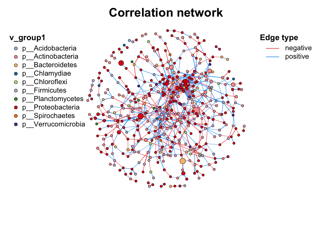
get_n(co_net)
##   n_type
## 1 single
# get vertex attributes
get_v(co_net) %>% head(5)
##                           name  v_group  v_class size
## 1 s__un_f__Thermomonosporaceae v_group1 v_class1    4
## 2        s__Pelomonas_puraquae v_group1 v_class1    4
## 3     s__Rhizobacter_bergeniae v_group1 v_class1    4
## 4     s__Flavobacterium_terrae v_group1 v_class1    4
## 5         s__un_g__Rhizobacter v_group1 v_class1    4
##                          label  shape   color
## 1 s__un_f__Thermomonosporaceae circle #a6bce3
## 2        s__Pelomonas_puraquae circle #a6bce3
## 3     s__Rhizobacter_bergeniae circle #a6bce3
## 4     s__Flavobacterium_terrae circle #a6bce3
## 5         s__un_g__Rhizobacter circle #a6bce3
# get edge attributes
get_e(co_net) %>% head(5)
##   id                         from                            to    weight
## 1  1 s__un_f__Thermomonosporaceae     s__Actinocorallia_herbida 0.6759546
## 2  2 s__un_f__Thermomonosporaceae       s__Kribbella_catacumbae 0.6742386
## 3  3 s__un_f__Thermomonosporaceae       s__Kineosporia_rhamnosa 0.7378741
## 4  4 s__un_f__Thermomonosporaceae   s__un_f__Micromonosporaceae 0.6236449
## 5  5 s__un_f__Thermomonosporaceae s__Flavobacterium_saliperosum 0.6045747
##         cor      p.value   e_type     width   color  e_class lty
## 1 0.6759546 0.0020739524 positive 0.6759546 #48A4F0 e_class1   1
## 2 0.6742386 0.0021502138 positive 0.6742386 #48A4F0 e_class1   1
## 3 0.7378741 0.0004730567 positive 0.7378741 #48A4F0 e_class1   1
## 4 0.6236449 0.0056818984 positive 0.6236449 #48A4F0 e_class1   1
## 5 0.6045747 0.0078660171 positive 0.6045747 #48A4F0 e_class1   1

And we can see, some attributes have been set when we build the network like v_group, these are internal attributes of metanet and are related to the following analysis and visualization.

Table 3.1: Internal attributes of a metanet

Attribute name	Description
v_group	the big group for network, usually one omics data produces one group. Related to the vertex shape.
v_class	some annotation of vertex, maybe classification or network modules. Related to the vertex color.
size	numeric variable assign to the vertex size.
e_type	the type of edges, often be the positive or negative according to correlation. Related to the edge color.
width	numeric variable assign to the edge width.
e_class	the second type of edges, often be the intra or inter according to two vertex group. Related to the edge line type.

We will talk about how to set these attributes for some specific analysis later.

3.2 Annotation

Sometimes we have lots of annotation tables need to add to the network, such as abundance table, taxonomy table and so on, we can use c_net_annotate() to do this.

The annotation dataframe needs have rowname or a “name” column which match the vertex name of metanet, c_net_annotate(mode = "v") or anno_vertex() will automatically match the vertex name and combine the table.

c_net_annotate(co_net, taxonomy["Phylum"], mode = "v") -> co_net1
get_v(co_net1) %>% head(5)
##                           name  v_group  v_class size
## 1 s__un_f__Thermomonosporaceae v_group1 v_class1    4
## 2        s__Pelomonas_puraquae v_group1 v_class1    4
## 3     s__Rhizobacter_bergeniae v_group1 v_class1    4
## 4     s__Flavobacterium_terrae v_group1 v_class1    4
## 5         s__un_g__Rhizobacter v_group1 v_class1    4
##                          label  shape   color            Phylum
## 1 s__un_f__Thermomonosporaceae circle #a6bce3 p__Actinobacteria
## 2        s__Pelomonas_puraquae circle #a6bce3 p__Proteobacteria
## 3     s__Rhizobacter_bergeniae circle #a6bce3 p__Proteobacteria
## 4     s__Flavobacterium_terrae circle #a6bce3  p__Bacteroidetes
## 5         s__un_g__Rhizobacter circle #a6bce3 p__Proteobacteria

c_net_annotate(mode = "e") or anno_edge() receives the same format annotation dataframe, it will automatically match the “from” and “to” columns so that you can summary the links.

anno <- data.frame("from" = "s__un_f__Thermomonosporaceae", "to" = "s__Actinocorallia_herbida", new_atr = "new")
c_net_annotate(co_net, anno, mode = "e") -> co_net1
get_e(co_net1) %>% head(5)
##   id                         from                            to    weight
## 1  1 s__un_f__Thermomonosporaceae     s__Actinocorallia_herbida 0.6759546
## 2  2 s__un_f__Thermomonosporaceae       s__Kribbella_catacumbae 0.6742386
## 3  3 s__un_f__Thermomonosporaceae       s__Kineosporia_rhamnosa 0.7378741
## 4  4 s__un_f__Thermomonosporaceae   s__un_f__Micromonosporaceae 0.6236449
## 5  5 s__un_f__Thermomonosporaceae s__Flavobacterium_saliperosum 0.6045747
##         cor      p.value   e_type     width   color  e_class lty new_atr
## 1 0.6759546 0.0020739524 positive 0.6759546 #48A4F0 e_class1   1     new
## 2 0.6742386 0.0021502138 positive 0.6742386 #48A4F0 e_class1   1    <NA>
## 3 0.7378741 0.0004730567 positive 0.7378741 #48A4F0 e_class1   1    <NA>
## 4 0.6236449 0.0056818984 positive 0.6236449 #48A4F0 e_class1   1    <NA>
## 5 0.6045747 0.0078660171 positive 0.6045747 #48A4F0 e_class1   1    <NA>

MetaNet provides function c_net_set() for easily annotation when you have more than one annotation table (it’s normal when you do a multi-omics analysis).

Abundance_df <- data.frame("Abundance" = colSums(totu))
# two annotation tables for vertex at same time, the rownames of Abundance_df and taxonomy do not need to be the same.
co_net1 <- c_net_set(co_net, taxonomy["Phylum"], Abundance_df)

get_v(co_net1) %>% head(5)
##                           name  v_group  v_class size
## 1 s__un_f__Thermomonosporaceae v_group1 v_class1    4
## 2        s__Pelomonas_puraquae v_group1 v_class1    4
## 3     s__Rhizobacter_bergeniae v_group1 v_class1    4
## 4     s__Flavobacterium_terrae v_group1 v_class1    4
## 5         s__un_g__Rhizobacter v_group1 v_class1    4
##                          label  shape   color            Phylum Abundance
## 1 s__un_f__Thermomonosporaceae circle #a6bce3 p__Actinobacteria     26147
## 2        s__Pelomonas_puraquae circle #a6bce3 p__Proteobacteria     25217
## 3     s__Rhizobacter_bergeniae circle #a6bce3 p__Proteobacteria     16592
## 4     s__Flavobacterium_terrae circle #a6bce3  p__Bacteroidetes     16484
## 5         s__un_g__Rhizobacter circle #a6bce3 p__Proteobacteria     13895

Note

If you have a vector and you absolutely know it matches the vertex name of network, you can use igraph method to annotate (Don’t recommend), same as the edge annotate vector. Refer to the igraph manual for more details.

co_net1 <- co_net

# add vertex attribute
V(co_net1)$new_attri <- seq_len(length(co_net1))
get_v(co_net1) %>% head(5)
##                           name  v_group  v_class size
## 1 s__un_f__Thermomonosporaceae v_group1 v_class1    4
## 2        s__Pelomonas_puraquae v_group1 v_class1    4
## 3     s__Rhizobacter_bergeniae v_group1 v_class1    4
## 4     s__Flavobacterium_terrae v_group1 v_class1    4
## 5         s__un_g__Rhizobacter v_group1 v_class1    4
##                          label  shape   color new_attri
## 1 s__un_f__Thermomonosporaceae circle #a6bce3         1
## 2        s__Pelomonas_puraquae circle #a6bce3         2
## 3     s__Rhizobacter_bergeniae circle #a6bce3         3
## 4     s__Flavobacterium_terrae circle #a6bce3         4
## 5         s__un_g__Rhizobacter circle #a6bce3         5

# add edge attribute
E(co_net1)$new_attri <- "new attribute"
get_e(co_net1) %>% head(5)
##   id                         from                            to    weight
## 1  1 s__un_f__Thermomonosporaceae     s__Actinocorallia_herbida 0.6759546
## 2  2 s__un_f__Thermomonosporaceae       s__Kribbella_catacumbae 0.6742386
## 3  3 s__un_f__Thermomonosporaceae       s__Kineosporia_rhamnosa 0.7378741
## 4  4 s__un_f__Thermomonosporaceae   s__un_f__Micromonosporaceae 0.6236449
## 5  5 s__un_f__Thermomonosporaceae s__Flavobacterium_saliperosum 0.6045747
##         cor      p.value   e_type     width   color  e_class lty     new_attri
## 1 0.6759546 0.0020739524 positive 0.6759546 #48A4F0 e_class1   1 new attribute
## 2 0.6742386 0.0021502138 positive 0.6742386 #48A4F0 e_class1   1 new attribute
## 3 0.7378741 0.0004730567 positive 0.7378741 #48A4F0 e_class1   1 new attribute
## 4 0.6236449 0.0056818984 positive 0.6236449 #48A4F0 e_class1   1 new attribute
## 5 0.6045747 0.0078660171 positive 0.6045747 #48A4F0 e_class1   1 new attribute

3.3 Set attributes

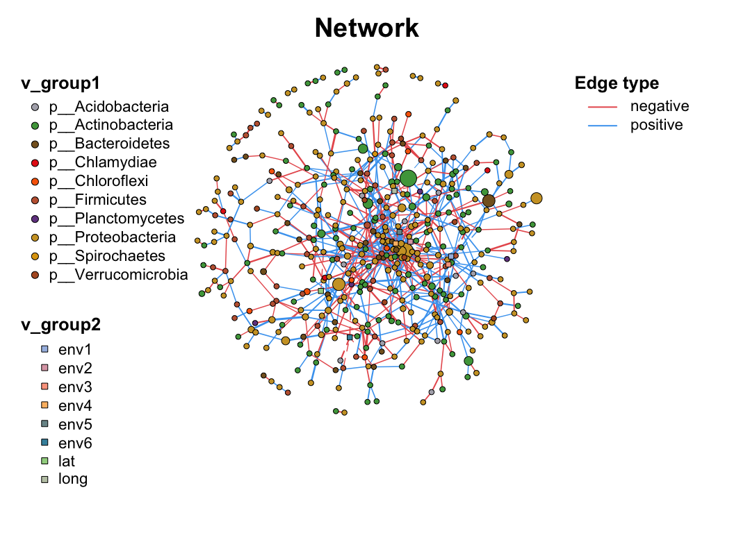
As we mentioned before, there are some internal attributes have been set when building network, which are related to the network visualization (Table 3.1). So we can use c_net_set() to custom these attributes fitting to our research needs.

Give the network various annotate tables and determine which columns use to set, we can give the columns name (one or more) to vertex_group, vertex_class, vertex_size, edge_type, edge_class, edge_width.

And the colors, linetypes, shapes and legends will be assigned automatically, just use plot() to get the basic metanet figure. For more details to customize the plot, refer to the next section: Chapter 4.

data("multi_test", package = "MetaNet")
data("c_net", package = "MetaNet")
# build a multi-network
multi1 <- multi_net_build(list(Microbiome = micro, Metabolome = metab, Transcriptome = transc))

plot(multi1)

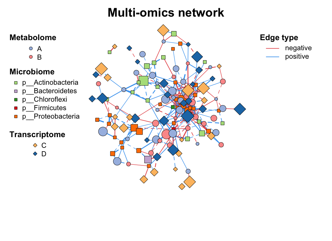
# set vertex_class
multi1_with_anno <- c_net_set(multi1, micro_g, metab_g, transc_g, vertex_class = c("Phylum", "kingdom", "type"))
# set vertex_size
multi1_with_anno <- c_net_set(multi1_with_anno,
  data.frame("Abundance1" = colSums(micro)),
  data.frame("Abundance2" = colSums(metab)),
  data.frame("Abundance3" = colSums(transc)),
  vertex_size = paste0("Abundance", 1:3)
)

plot(multi1_with_anno)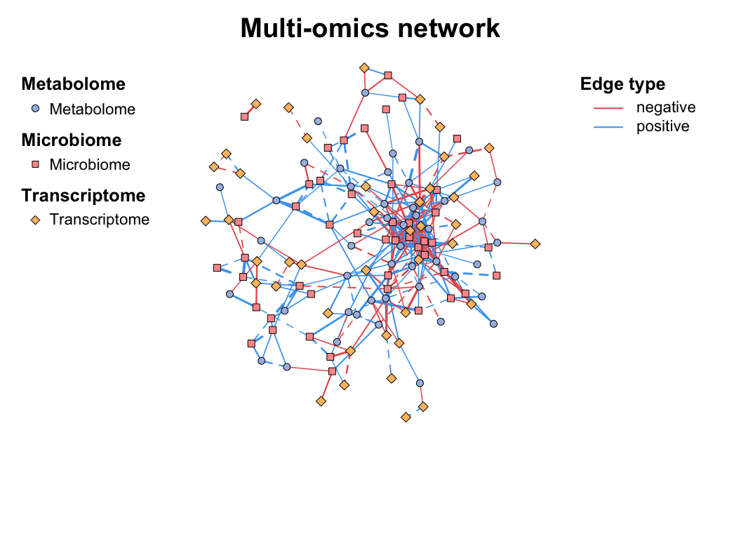

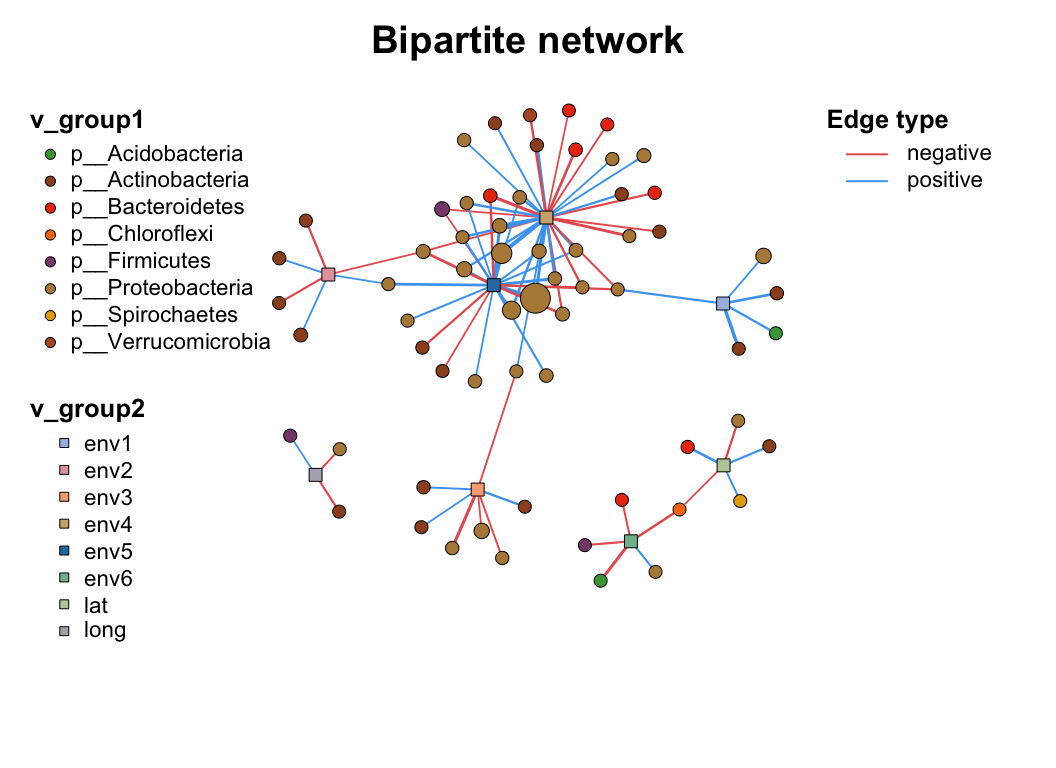
3.4 Filter (Sub-net)

After setting your network properly, you may need to analysis part of the whole network (especially in the multi-omics analysis), c_net_filter() can get the sub-net conveniently, you can put lots of filter conditions (like the dplyr::filter) and get the sub-net you want.

data("multi_net", package = "MetaNet")
multi2 <- c_net_filter(multi1_with_anno, v_group %in% c("Microbiome", "Metabolome")) %>%
  c_net_filter(., e_class == "intra", mode = "e")

par(mfrow = c(2, 1))
plot(multi1_with_anno, lty_legend = T, main = "Before filtering network") # before filter
plot(multi2, lty_legend = T, main = "After filtering network") # after filter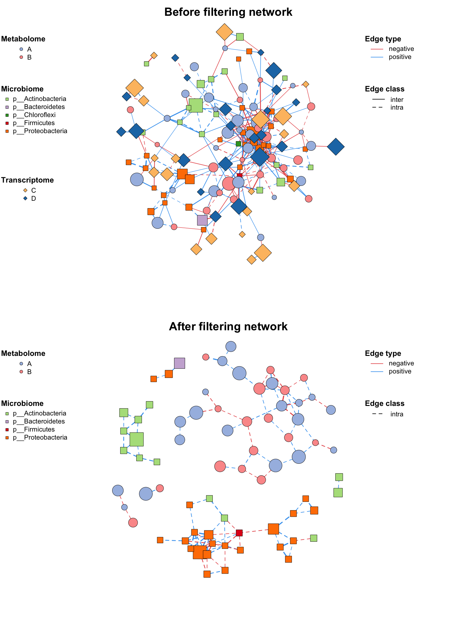

3.5 Union (Combine)

If you have two networks and want to combine them, you can use c_net_union().

data("c_net")
plot(co_net)
plot(co_net2)

co_net_union <- c_net_union(co_net, co_net2)
plot(co_net_union)

3.6 Skeleton

If you want to summary the edges source and target according to one group, summ_2col is a easy way to get this information.

direct = F argument means this is a undirected relationship, so “a-b” and “b-a” will summary to one type edge.

c_net_annotate(co_net, select(taxonomy, "Phylum"), mode = "e") -> co_net1
df <- get_e(co_net1)[, c("Phylum_from", "Phylum_to")]
summ_2col(df, direct = F) %>% arrange(-count) -> Phylum_from_to

kbl(Phylum_from_to, caption = "Summary of edges according to Phylum") %>%
  kable_paper() %>%
  scroll_box(width = "100%", height = "400px")

Summary of edges according to Phylum
Phylum_from	Phylum_to	count
p__Proteobacteria	p__Proteobacteria	210
p__Actinobacteria	p__Proteobacteria	161
p__Firmicutes	p__Proteobacteria	63
p__Actinobacteria	p__Actinobacteria	62
p__Bacteroidetes	p__Proteobacteria	54
p__Actinobacteria	p__Firmicutes	34
p__Actinobacteria	p__Bacteroidetes	25
p__Acidobacteria	p__Proteobacteria	21
p__Proteobacteria	p__Verrucomicrobia	13
p__Bacteroidetes	p__Firmicutes	11
p__Firmicutes	p__Firmicutes	10
p__Chloroflexi	p__Proteobacteria	9
p__Actinobacteria	p__Chloroflexi	8
p__Planctomycetes	p__Proteobacteria	7
p__Acidobacteria	p__Actinobacteria	6
p__Actinobacteria	p__Verrucomicrobia	5
p__Bacteroidetes	p__Bacteroidetes	5
p__Chlamydiae	p__Proteobacteria	5
p__Chloroflexi	p__Firmicutes	5
p__Bacteroidetes	p__Verrucomicrobia	4
p__Actinobacteria	p__Planctomycetes	3
p__Proteobacteria	p__Spirochaetes	3
p__Acidobacteria	p__Chloroflexi	2
p__Actinobacteria	p__Chlamydiae	2
p__Actinobacteria	p__Spirochaetes	2
p__Chloroflexi	p__Verrucomicrobia	2
p__Acidobacteria	p__Firmicutes	1
p__Acidobacteria	p__Verrucomicrobia	1
p__Bacteroidetes	p__Chloroflexi	1
p__Bacteroidetes	p__Spirochaetes	1
p__Chlamydiae	p__Firmicutes	1
p__Chlamydiae	p__Spirochaetes	1
p__Firmicutes	p__Planctomycetes	1
p__Firmicutes	p__Verrucomicrobia	1

Then you can use sankey plot to display the links.

pcutils::my_sankey(Phylum_from_to, dragY = T, fontSize = 10, width = 600, numberFormat = ",.4")

Figure 3.4: Sankey plot display edges according to Phylum

Or use the circlize plot to display. link_stat() have more arguments than summ_2col() for summary edges.

c_net_set(co_net, select(taxonomy, "Phylum")) -> co_net1
links_stat(co_net1, topN = 5, group = "Phylum", e_type = "all")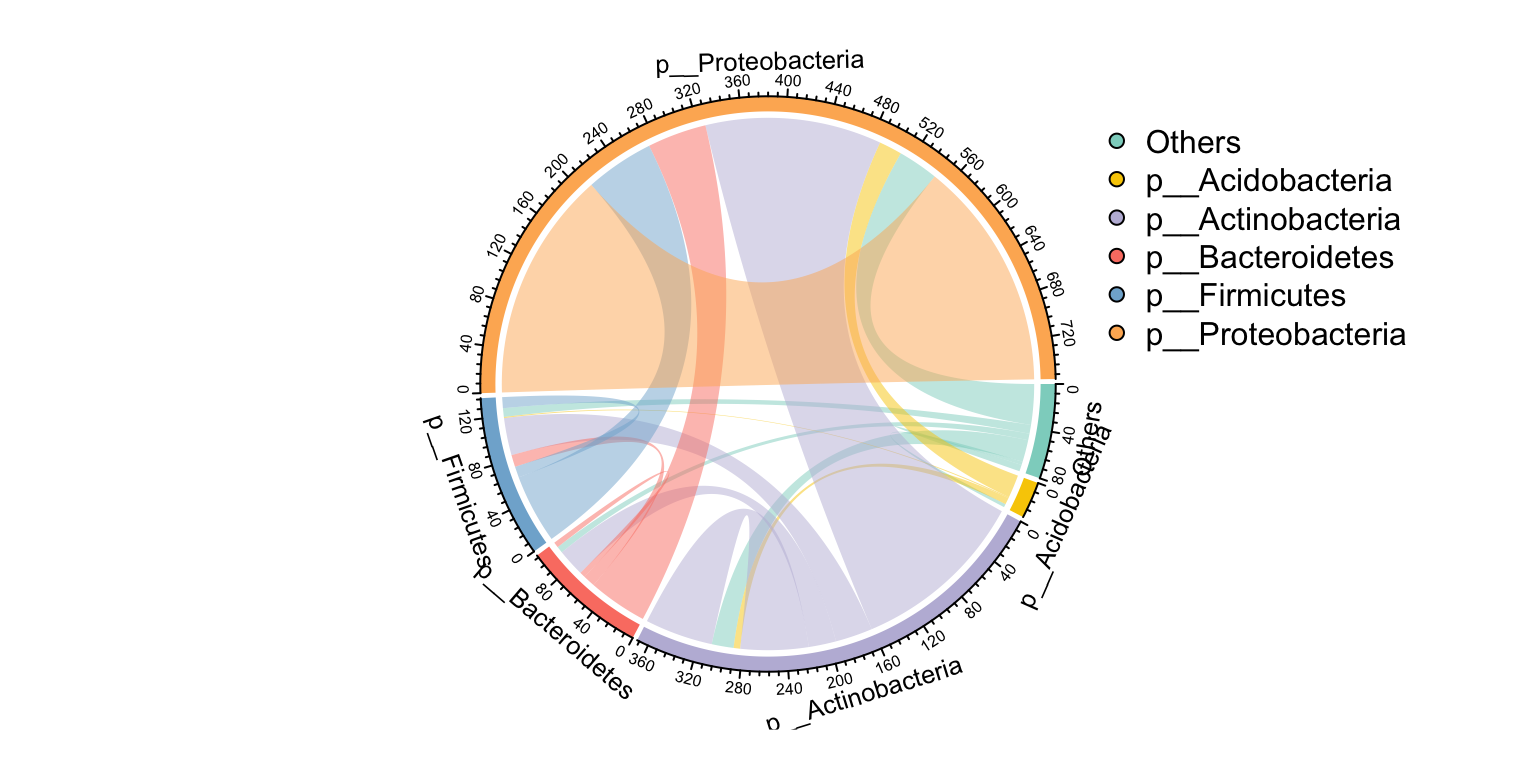

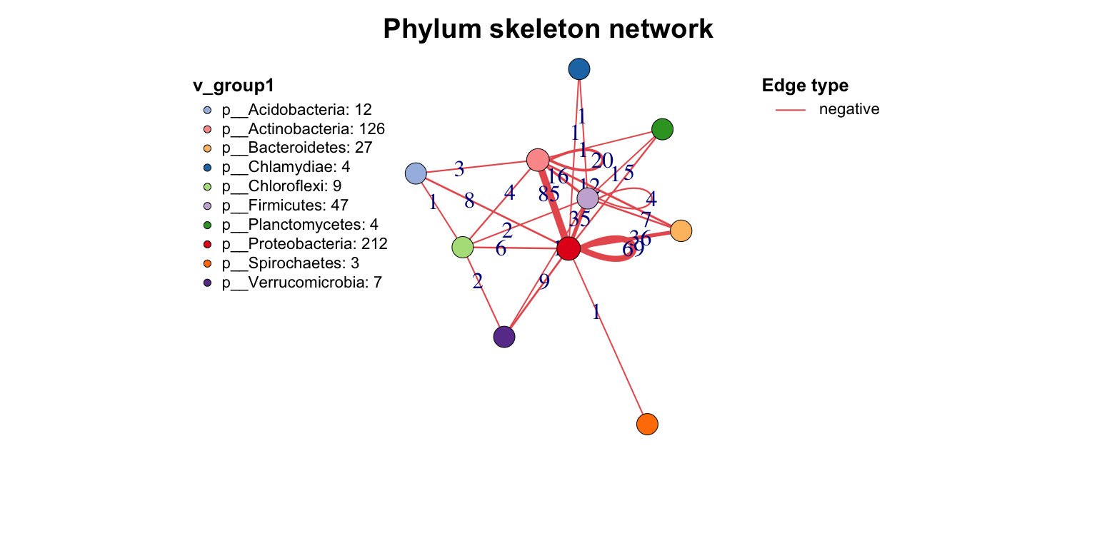
Figure 3.5: Circlize plot display edges according to Phylum

Other important action for a network is extracting the skeleton according to one group, which I call get skeleton plot. get_group_skeleton() can annotate all nodes with a group then combine each group nodes as a big node, and calculate new links between all groups.

This plot shows the flows between different groups clearly. By the way, the result will display by different edge types, if you just want summary all edges, set the e_type as one same character (use c_net_set()).

get_group_skeleton(co_net1, Group = "Phylum") -> ske_net
plot(ske_net, vertex.label = NA)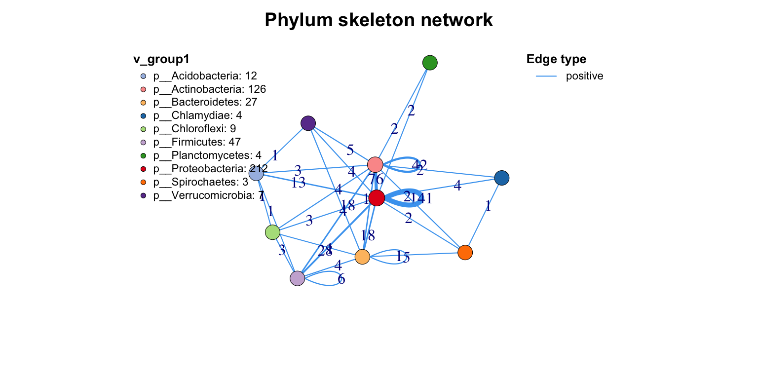

Figure 3.6: Skeleton plot according to the Phylum

Figure 3.7: Skeleton plot according to the Phylum

3.7 Save

MetaNet also support to export various format network files (data.frame, graphml, pajek, lgl, …) for following analysis in other softwares (Cytoscape, Gephi…). You can use c_net_save() to save the network as a file, and use c_net_load() to load the network from a file.

c_net_save(co_net, filename = "My_net", format = "data.frame")
c_net_save(co_net, filename = "My_net", format = "graphml")

c_net_load("My_net.graphml")