Chapter 12 Laboratory 4: Dendrochronology and Climate
12.1 Introduction
In recent lectures, we have discussed the climate history of Earth, as well as global climate change. One of the aspects of studying climate is the subfield of paleoclimatology (paleo meaning “older”), which uses a variety of methods to infer past climate history. These methods include work on ice cores, coral rings, and tree rings. It is important to study our paleoclimate because if we can make current models of the earth’s climate operate well using good past climate data, it may be possible to accurately predict future climate. Unfortunately, our direct measurements of climate are historically, relatively short (the longest we have even semi-global temperature records for is about 150 years) and spatially, quite sparse. The learning objectives of this laboratory exercise are to learn how to core trees, to learn to date your tree cores using common computer packages, and to hone your comparative analysis skills.
Dendrochronology (also known as tree-ring dating) is dating based on the analysis of tree rings. During the growth of a tree, a layer of wood cells is produced under the bark—as such, each layer is a ring that represents a particular year’s growth. The width or thickness of these rings is one of the measurements used in dendrochronology. With advanced approaches (beyond what you will do), this particular method can be used to date wood back many thousands of years.
There are many implications behind measuring the thickness of tree rings, with the most immediate being its usage as an indicator, or proxy, for past climatic conditions. When climatic conditions are optimal for tree growth, trees will grow more and rings will be wider. With poor growing conditions, the opposite is true. Tree growth is particularly sensitive to moisture availability (precipitation is a strong control on soil moisture), but climatic variables like temperature and cloud cover (trees are dependent on light for photosynthesis of course) also play an important role in tree growth. In reality, dendroclimatic relationships work best when the tree being used is most often under some sort of climate-related stress (e.g., grows in a normally drought-ridden environment).
You will first visit the forest plot across the road from the lab building to see how trees are cored. Then, in groups of 4 or 5 students and using tree cores archived from last year, you will conduct an imaging analysis of your tree core, “standardize” your values and relate your standardized values and their chronology to local, relatively long-term climate records.
Although you are working in groups to obtain data, your assignment must be completed individually.
12.2 Safety Concern
The cutting end of an increment borer is extremely sharp. Treat it the same as you would a sharp knife in your kitchen because it will slice through skin just as easily. If you somehow cut yourself while in the field, notify your TA immediately.
12.3 Procedure for Laboratory 4
Follow your TA to the forest plot across from the lab building where they will demonstrate how to core a tree.
In groups and using a flexible tape, measure the diameter at breast height (DBH) of 5 random trees in the forest. Record these in your notebook.
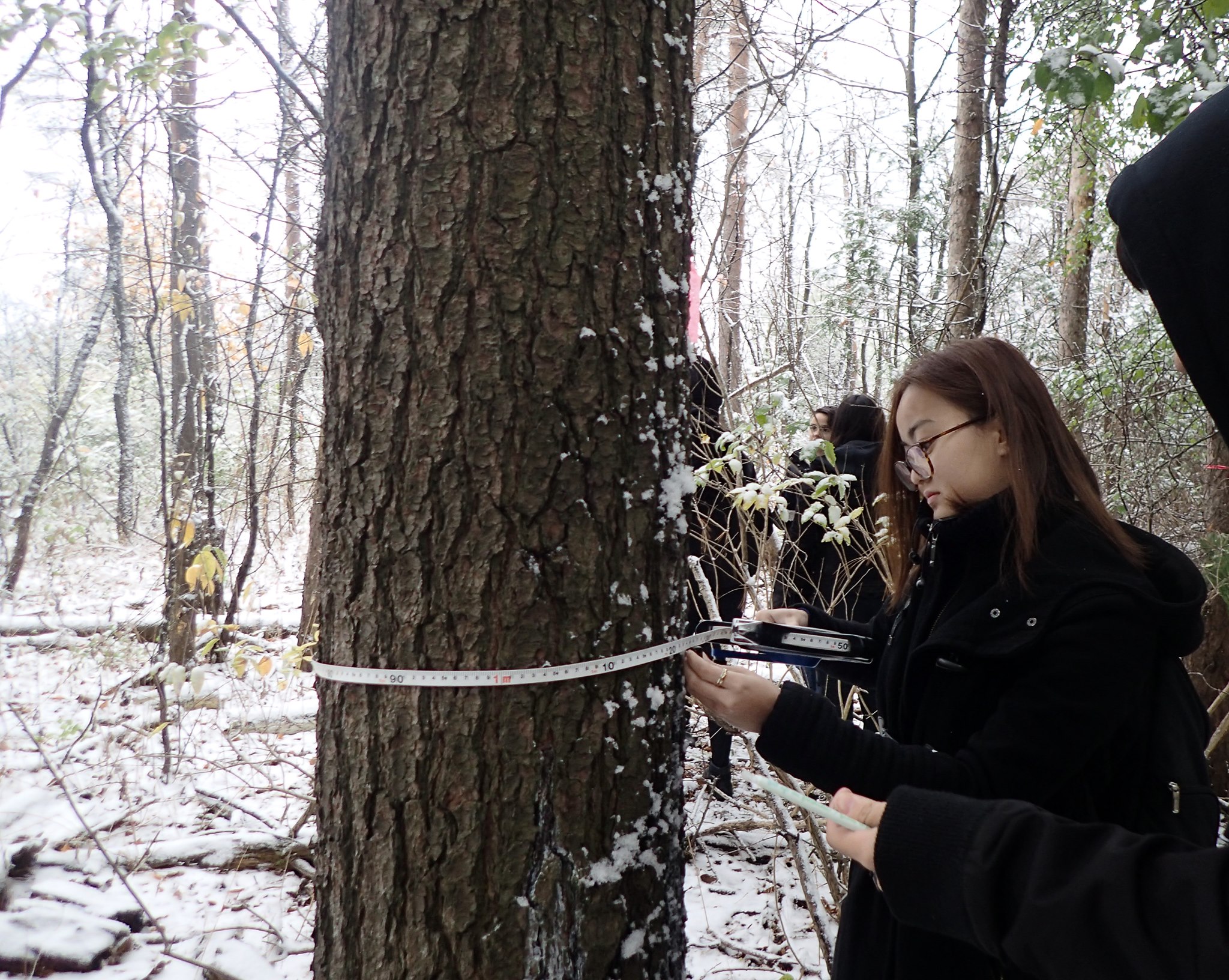
Plate 12.1: Students measuring the DBH of a tree. Photo taken by Tom Meulendyk and Chai Chen. Click here for source
Each group will also get a chance to extract one tree core. The tree core you extract is NOT used for this lab. You and your group can decide what to do with the tree core once it is extracted.
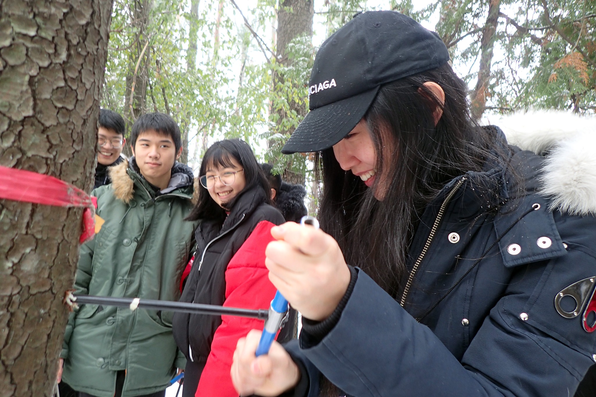
Plate 12.2: A student using an increment borer. Photo taken by Tom Meulendyk and Chai Chen. Click here for source
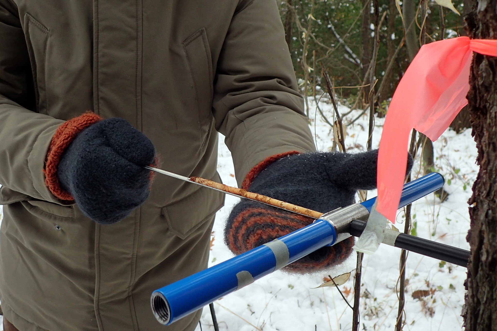
Plate 12.3: A tree core. Photo taken by Tom Meulendyk and Chai Chen. Click here for source
Obtain an archived core from your TA and work on the remainder of data collection in groups of 4-5.
Place your core into the scanner face down and scan your core at 2400 DPI. Save this image and name it accordingly, as you will be using this to conduct your tree ring analysis in CooRecorder and CDendro software. Save a copy of the image for yourself somehow so you can include it in your assignment.
Open CooRecorder. Click on File in the menu bar and select the option to “Open image file for new coordinates.” Select and open the image that you had just scanned.
Set the DPI value to be 1200. Once imported, CooRecorder will show your image as below.
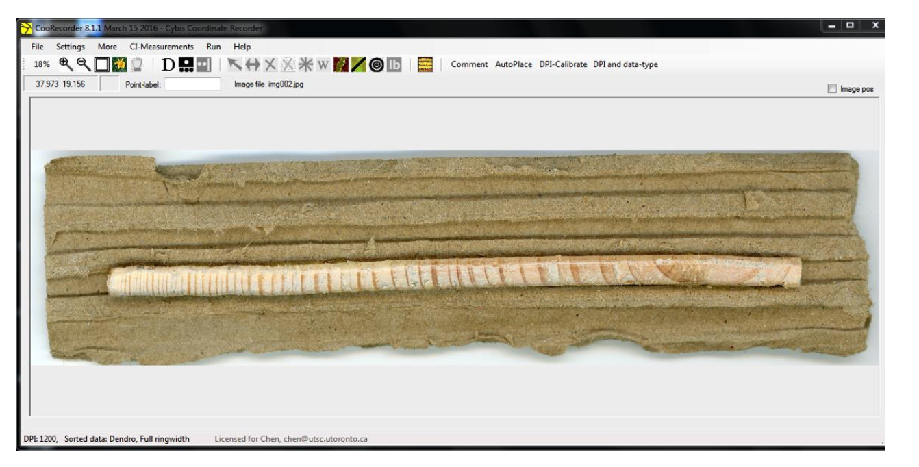
Figure 12.1: What the prepared tree core looks like.
- Using the help-line button, place a point outside the youngest ring, and then a second point just before the middle of the pith. An example is shown below.

Figure 12.2: The help-line button.
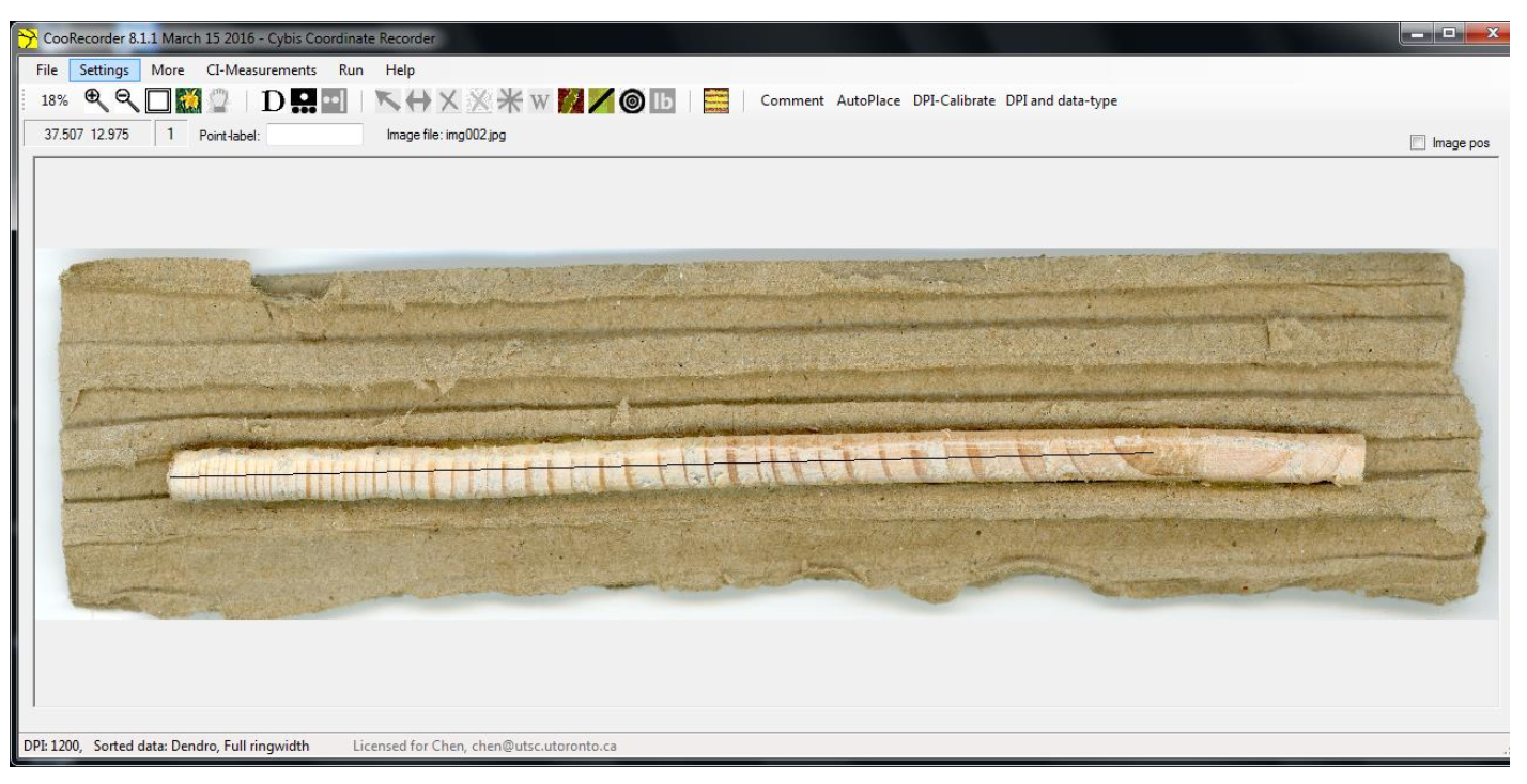
Figure 12.3: Example of a placed help-line.
- Once your help-line is placed, select the AutoPlace option. Similar to the previous step, trace your help-line by placing the two points on the same locations in the same order. This will automatically place points on most of your tree rings, but not all of them, as shown below.

Figure 12.4: The AutoPlace button.
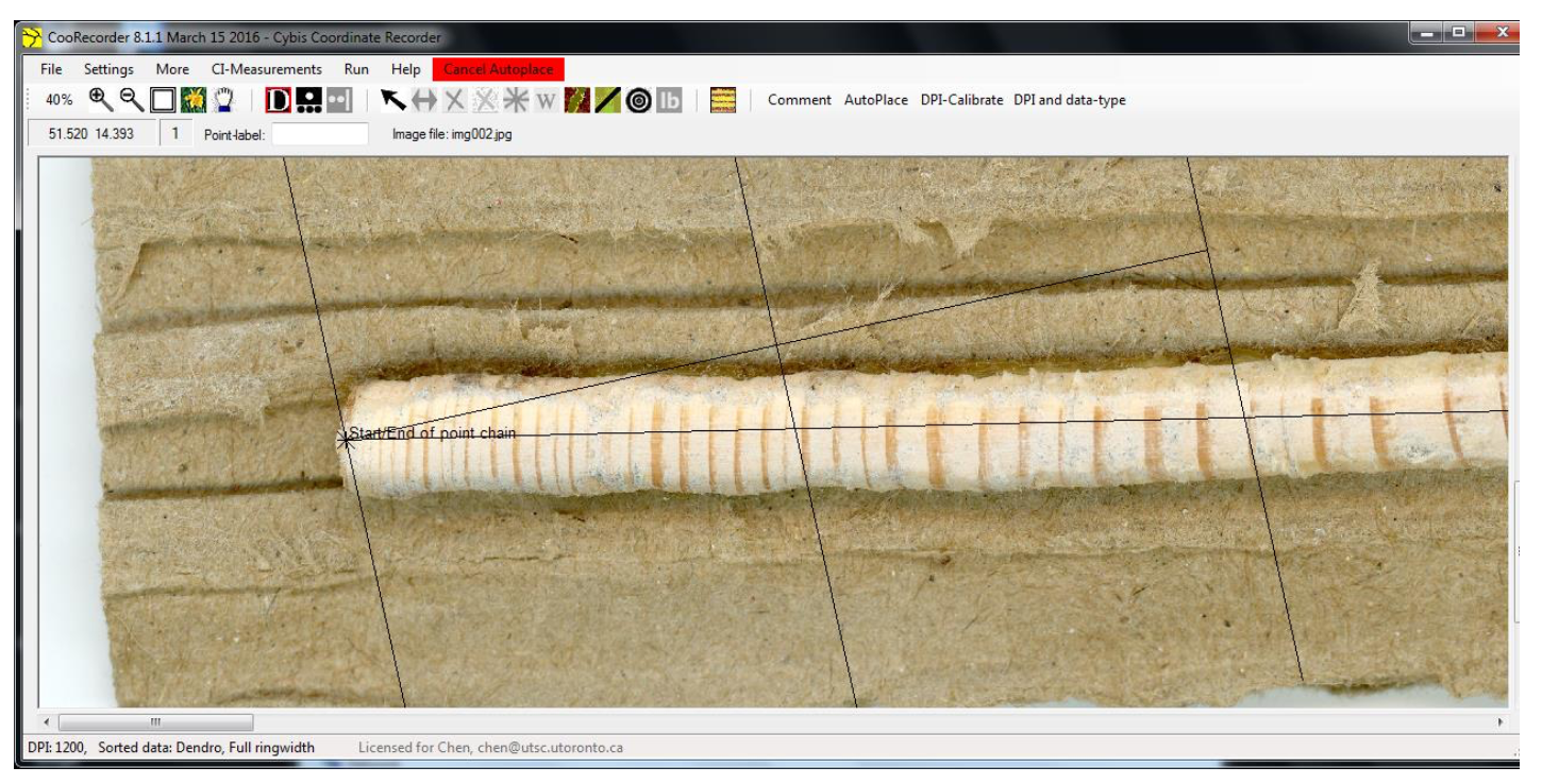
Figure 12.5: Selecting the first point for AutoPlace.
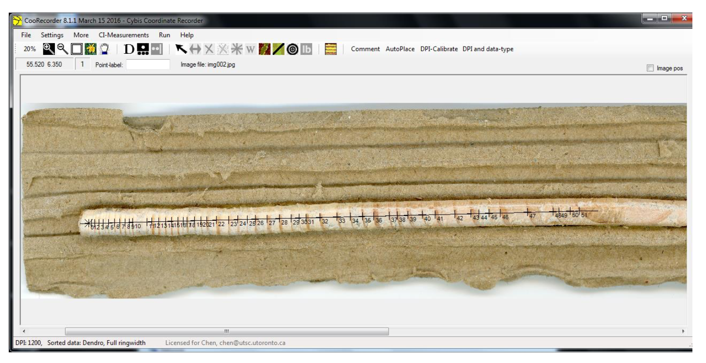
Figure 12.6: Completed AutoPlace. Note the finishing position before the pith, but after the oldest tree ring.
- Zoom in closer so you have a more accurate view of the tree rings. From this point, you will have to manually select the tree rings that AutoPlace may not have detected. Using the Data picking mode, select the youngest tree ring that was not detected. If this ring is outside what AutoPlace had detected, you will likely encounter an error as shown in Figure 12.9 below (if the error does not occur and your rings appear to be in order, continue with step 12). To correct this, ensure that the point you placed is highlighted, and then click on the start point button. This will alter the order of points so that your highlighted point becomes number 1, and is the youngest.
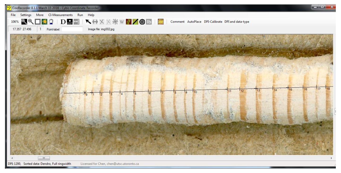
Figure 12.7: Zoomed in view showing missed data points.
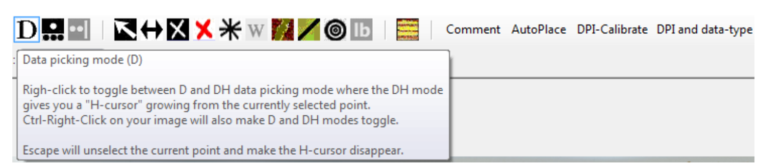
Figure 12.8: Data picking mode.
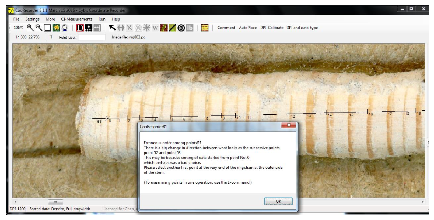
Figure 12.9: Error when placing a data point before the initial point in AutoPlace.
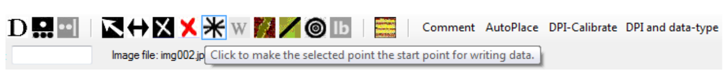
Figure 12.10: Button to make selected point the starting point.
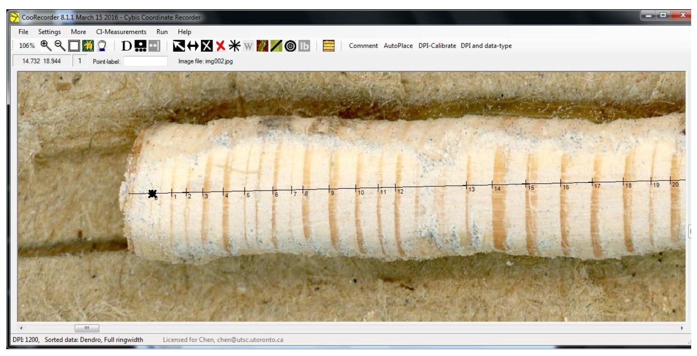
Figure 12.11: Correction of tree ring order.
- After you have corrected your order, you can resume placing missed points with the data picking mode.
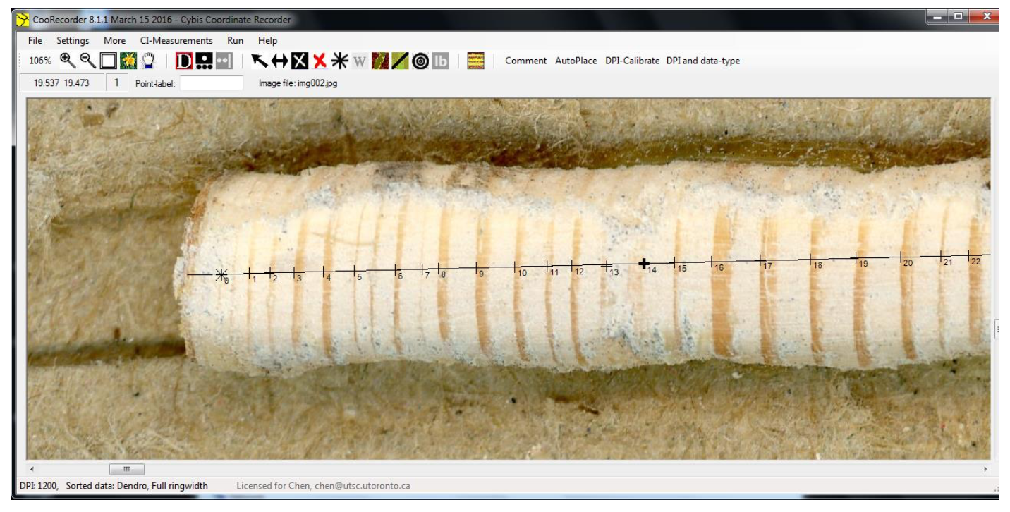
Figure 12.12: Placing the missed points through data picking mode.
- Once you have placed all the points for the missing tree rings, it is time to define distance to pith. Select the distance to pith button and select “Ok, define now!” in the window that appears. At this point, a moveable overlay with concentric layers will appear—you will attempt to match this as closely to your tree core as possible, estimating where the pith is. Once you have found a suitable point for your pith, click on that point. A window titled “Estimating Years to Pith” will pop up. Leave the estimation of Years to Pith at 1, and select OK.

Figure 12.13: Set distance to pith button.
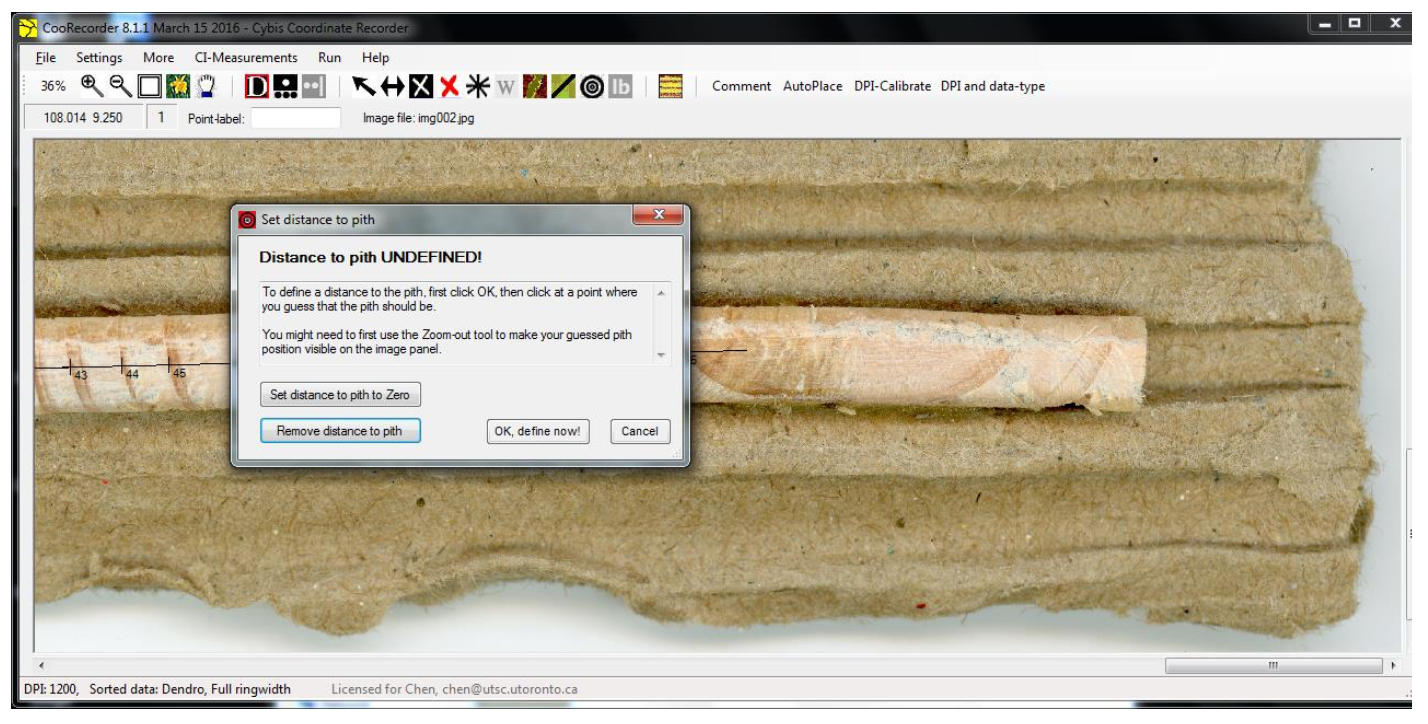
Figure 12.14: Setting up to define the distance to pith.
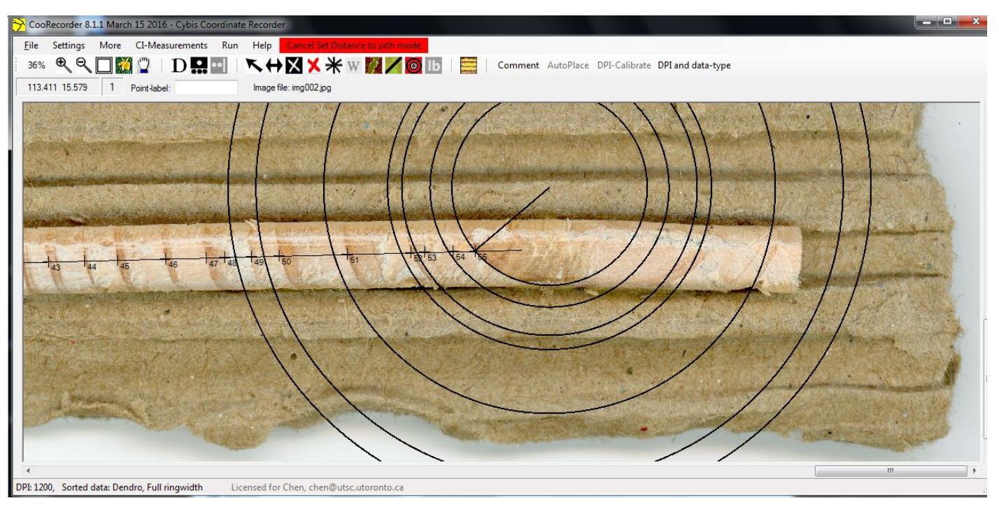
Figure 12.15: Defining the pith’s location and distance to pith.
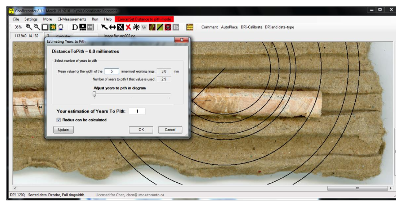
Figure 12.16: Verifying the pith distance and estimate of years to pith.
You can now save your file by clicking on File in the menu and selecting the option to “Save coordinate file.” Save this file as a .pos file and name it accordingly.
Open CDendro and open your coordinate file by clicking on Sample in the menu and select “Open one or more single sample files: .pos, .wid, .datw, .cat, .d, .crn.” Select the .pos coordinate file you had just saved with CooRecorder.
Under the Curve display tab, you will see your data in the form of a graph. Hit the fit to screen button, and it will expand your graph to properly fit the horizontal axis. At this point, hovering over any of the numbered data points will give you the respective widths of the rings. Take a screen shot of this image and save it for your later use. Your TA will also show you how to export your data for use in the assignment.
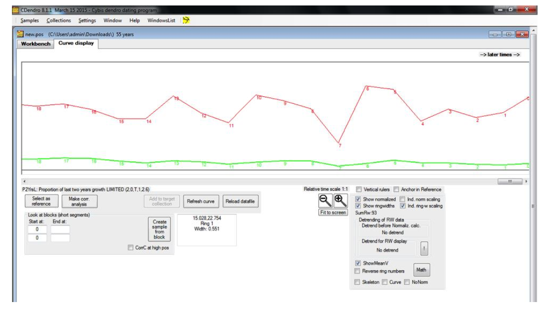
Figure 12.17: An example of the output you should expect after opening your file in CDendro.
Make sure you have finished the following before you exit the laboratory:
- You have circumference measurements for 5 individual trees
- You have a photo of your tree core
- You have a photo of the tree ring width analysis from the CDendro software (i.e., procedure point #14 above).
- You have exported the data from the CDendro program (procedure point #14 above)
- You have cleaned up your work area
12.4 Assignment #4
Assignment 4 is 41 marks total – worth 10% of your final grade.
This is your FINAL LAB ASSIGNMENT. This assignment will be submitted online ONLY. Please submit a pdf version of your assignment on Quercus under “Lab 4 submission”. See Quercus for when Lab 4 is due.
What are the DBH of the individual trees your measured and give the mean DBH of the 5 trees? Provide a photo of your tree core (i.e., procedure point #4). Using your archived core, state how many years that tree has the tree been growing for? The tree cores were extracted in the year 2016, so please remember to add the difference in time between then and now. (5 marks)
Provide a photo of the tree ring width analysis from the CDendro software (i.e., procedure point #14 above). In two sentences or less, broadly describe the patterns you see. Why do you suspect you see this pattern? (5 marks)
Because of your answer to #2, there is a clear bias in your data. You will therefore need to “standardize” your data. To do this:
- Using your spreadsheet, “fit” an exponential decay trendline to your ring width vs. year data. Properly label the graph and include the equation on it (hand this in as part of your answer to this question). The equation should be of the form y = a\(e\)-bx. (5 marks)
In your spreadsheet of ring width vs.year data,add a new column titled “trend”. To calculate these values, use your equation from question 3 and the year data (x- axis data) to solve for y for each year. Copy and paste this for every year. Add another new column and call it “deviation from trend”. To calculate the numbers in this column, simply subtract the “trend” number from your actual ring width – copy and paste this for every year. Fit this table to one page and submit as your answer to question #4. (4 marks)
From Quercus, download the two files called “Toronto historical homogenized temp record.xlsx” and “Toronto historical homogenized precip record.xlsx”, which have annual means for temperature and total precipitation. Using the same duration that is covered by your tree core, construct a single time series graph showing both annual mean temperature and annual total precipitation throughout the duration that your tree ring covers. (8 marks)
Construct two different scatterplot graphs that display “deviation from trend” (from question 4) versus: (\(i\)) annual total precipitation and (\(ii\)) mean annual temperature over the duration of your tree ring record. Add a trendline to each graph, including an R2 value and a linear equation. (10 marks)
Comment on and compare the strengths of the relationships in question #6 and explain why the relationships are strong or weak (less than 10 lines). (4 marks)
You should have a written account of what you have done in a given experiment. Making detailed notes during the lab will help you in answering the questions in the assignment.