Chapter 9 GP Fidelity and Scale
Gaussian processes are fantastic, but they’re not without drawbacks. Computational complexity is one. Flops in \(\mathcal{O}(n^3)\) for matrix decompositions, furnishing determinants and inverses, is severe. Many practitioners point out that storage, which is in \(\mathcal{O}(n^2)\), is the real bottleneck, at least on modern laptops and workstations. Even if you’re fine with waiting hours for MVN density calculation for a single likelihood evaluation, chances are you wouldn’t have enough high-speed memory (RAM) to store the \(n \times n\) matrix \(\Sigma_n\), let alone its inverse too and any auxiliary space required. There’s some truth to this, but usually I find time to be the limiting factor. MLE calculations can demand hundreds of decompositions. Big memory supercomputing nodes are a thing, with orders of magnitude more RAM than conventional workstations. Big time nodes are not. Except when executions can be massively parallelized, supercomputers aren’t much faster than high-end laptops.
Although GP inference and prediction (5.2)–(5.3) more prominently feature inverses \(\Sigma_n^{-1}\), it’s actually determinants \(|\Sigma_n|\) that impose the real bottleneck. Both are involved in MVN density/likelihood evaluations. Conditional on hyperparameters, only \(\Sigma_n^{-1}\) is required. A clever implementation could solve the requisite system of equations for prediction, e.g., \(\Sigma_n^{-1} Y_n\) for the mean and \(\Sigma_n^{-1} \Sigma(X_n, x)\) for the variance, without explicitly calculating an inverse. Parallelization over elements of \(x \in \mathcal{X}\), extending to \(\Sigma_n^{-1} \Sigma(X_n, \mathcal{X})\), is rather trivial. All that sounds sensible and actionable, but actually it’s little more than trivia. Knowing good hyperparameters (without access to the likelihood) is “rare” to say the least. Let’s presume likelihood-based inference is essential and not pursue that line of thinking further. Full matrix decomposition is required.
Most folks would agree that Cholesky decomposition, leveraging symmetry in distance-based \(\Sigma_n\), offers the best path forward.9 The Cholesky can furnish both inverse and determinant in \(\mathcal{O}(n^3)\) time, and in some cases even faster depending on the libraries used. Divide-and-conquer parallelization also helps on multi-core architectures. I strongly recommend Intel MKL which is the workhorse behind Microsoft R Open on Linux and Windows, and the Accelerate Framework on OSX. Both provide conventional BLAS/LAPACK interfaces with modern implementations and customizations under the hood. An example of the potential with GP regression is provided in Appendix A. As explained therein, OpenBLAS is not recommended in this context because of thread safety issues which become relevant in nested, and further parallelized application (e.g., §9.3).
Ok, that’s enough preamble on cumbersome calculations. Computational complexity is one barrier; flexibility is another. Stationarity of covariance is a nice simplifying assumption, but it’s not appropriate for all data generating mechanisms. There are many ways data can be nonstationary. The LGBB rocket booster (see §2.1), whose simulations are deterministic, exhibits mean nonstationarity along with rather abrupt regime changes from steep to flat dynamics. When data/simulations are noisy, variance nonstationarity or heteroskedasticity may be a concern: noise levels which are input-dependent. Changes in either may be smooth or abrupt. GPs don’t cope well in such settings, at least not in their standard form. Enhancing fidelity in GP modeling, to address issues like mean and variance nonstationarity, is easy in theory: just choose a nonstationary kernel. In practice it’s harder than that. What nonstationary kernel? What happens when regimes change and dynamics aren’t smooth?
Often the two issues, speed and flexibility, are coupled together. Coherent high-fidelity GP modeling schemes have been proposed, but in that literature there’s a tendency to exacerbate computational bottlenecks. Coupling processes together, for example to warp a nonstationary surface into one wherein simpler stationary dynamics reign (e.g., A. Schmidt and O’Hagan 2003; Sampson and Guttorp 1992) adds layers of additional computational complexity and/or requires MCMC. Consequently, such methods have only been applied on small data by modern standards. Yet observing complicated dynamics demands rich and numerous examples, putting data collection at odds with modeling goals. In a computer surrogate modeling context, where design and modeling go hand in hand, this state of affairs is particularly limiting. Surrogates must be flexible enough to drive sequential design acquisitions towards efficient learning, but computationally thrifty enough to solve underlying decision problems in time far less than it would take to run the actual simulations – a hallmark of a useful surrogate (§1.2.2).
This chapter focuses on GP methods which address those two issues, computational thrift and modeling fidelity, simultaneously. GPs can only be brought to bear on modern big data problems in statistics and machine learning (ML) by somehow skirting full dense matrix decomposition. There are lots of creative ways of doing that, some explicitly creating sparse matrices, some implicitly. Approximation is a given. A not unbiased selection of examples and references is listed below.
- Pseudo-inputs (Snelson and Ghahramani 2006) or the predictive process [PP; Banerjee et al. (2008)]; both examples of methods based on inducing points
- Iterating over batches (Haaland and Qian 2011) and sequential updating (Gramacy and Polson 2011)
- Fixed rank kriging (Cressie and Johannesson 2008)
- Compactly supported covariances and fast sparse linear algebra (Kaufman et al. 2011; Sang and Huang 2012)
- Partition models (Gramacy and Lee 2008a; Kim, Mallick, and Holmes 2005)
- Composite likelihood (Eidsvik et al. 2014)
- Local neighborhoods (Emery 2009; Gramacy and Apley 2015)
The literature on nonstationary modeling is more niche, although growing. Only a couple of the ideas listed above offer promise in the face of both computational and modeling challenges. This will dramatically narrow the scope of our presentation, as will the accessibility of public implementation in software.
There are a few underlying themes present in each of the approaches above: inducing points, sparse matrices, partitioning, and approximation. In fact all four can be seen as mechanisms for inducing sparsity in covariance. But they differ in how they leverage that sparsity to speed up calculations, and in how they offer scope for enhanced fidelity. It’s worth noting that you can’t just truncate as a means of inducing sparsity. Rounding small entries \(\Sigma^{ij}_n\) to zero will almost certainly destroy positive definiteness.
We begin in this chapter by illustrating a distance-based kernel which guarantees both sparsity and positive definiteness, however as a device that technique underwhelms. Sparse kernels compromise on long-range structure without gaining enhanced local modeling fidelity. Calculations speed up, but accuracy goes down despite valiant efforts to patch up long-range effects.
We then turn instead to implicit sparsity via partitioning and divide-and-conquer. These approaches, separately leveraging two key ideas from computer science – tree data structures on the one hand and transductive learning on the other – offer more control on speed versus accuracy fronts, which we shall see are not always at odds. The downside however is potential lack of smoothness and continuity. Although GPs are famous for their gracefully flowing surfaces and sausage-shaped error-bars, there are many good reasons to eschew that aesthetic when data get large and when mean and variance dynamics may change abruptly.
Finally, Chapter 10 focuses explicitly on variance nonstationarity, or input dependent noise, and low-signal scenarios. Stochastic simulations represent a rapidly growing sub-discipline of computer experiments. In that context, and when response surfaces are essential, tightly coupled active learning and GP modeling strategies (not unlike the warping ideas dismissed above) are quite effective thanks to a simple linear algebra trick, and generous application of replication as a tried and true design strategy for separating signal from noise.
9.1 Compactly supported kernels
A kernel \(k_{r_{\max}}(r)\) is said to have compact support if \(k_{r_{\max}}(r) = 0\) when \(r > r_{\max}\). Recall from §5.3.3 that \(r = |x - x'|\) for a stationary covariance. We may still proceed component-wise with \(r_j = |x_j - x_j'|\) and \(r_{j,\max}\) for a separable compactly supported kernel, augment with scales for amplitude adjustments, nuggets for noisy data and embellish with smoothness parameters (Matérn), etc. Rate of decay of correlation can be managed by lengthscale hyperparameters, a topic we shall return to shortly.
A compactly supported kernel (CSK) introduces zeros into the covariance matrix, so sparse matrix methods may be deployed to aid in computations, both in terms of economizing on storage and more efficient decomposition for inverses and determinants. Recall from §5.3.3 that a product of two kernels is a kernel, so a good way to build a bespoke CSK with certain properties is to take a kernel with those properties and multiply it by a CSK – an example of covariance tapering (Furrer, Genton, and Nychka 2006).
Two families of CSKs, Bohman and truncated power, offer decent approximations to the power exponential family (§5.3.3), of which the Gaussian (power \(\alpha=2\)) is a special case. These kernels are zero for \(r > r_{\max}\), and for \(r \leq r_{\max}\):
\[ \begin{aligned} k^{\mathrm{B}}_{r_{\max}}(r) &= \left(1-\frac{r}{r_{\max}}\right) \cos \left(\frac{\pi r}{r_{\max}}\right) + \frac{1}{\pi}\sin\left(\frac{\pi r}{r_{\max}}\right) \\ k^{\mathrm{tp}}_{r_{\max}}(r; \alpha, \nu) &= [1 - (r/r_{\max})^\alpha]^\nu, \quad \mbox{ where } 0 < \alpha < 2 \mbox{ and } \nu \geq \nu_m(\alpha). \end{aligned} \]
The function \(\nu_m(\alpha)\) in the definition of the truncated power kernel represents a restriction necessary to ensure a valid correlation in \(m\) dimensions, with \(\lim_{\alpha \rightarrow 2} \nu_m(\alpha) = \infty\). Although it’s difficult to calculate \(\nu_m(\alpha)\) directly, there are known upper bounds for a variety of \(\alpha\)-values between \(1.5\) and \(1.955\), e.g., \(v_1(3/2) \leq 2\) and \(v_1(5/3) \leq 3\). Chapter 9 of Wendland (2004) provides several other common CSKs. The presentation here closely follows Kaufman et al. (2011), concentrating on the simpler Bohman family as a representative case.
Bohman CSKs yield a mean-square differentiable process, whereas the truncated power family does not (unless \(\alpha = 2)\). Notice that \(r_{\max}\) plays a dual role, controlling both lengthscale and degree of sparsity. Augmenting with explicit lengthscales, i.e., \(r_\theta = r/\sqrt{\theta}\), enhances flexibility but at the expense of identifiability and computational concerns. Since CSKs are chosen over other kernels with computational thrift in mind, fine-tuning lengthscales often takes a back seat.
9.1.1 Working with CSKs
Let’s implement the Bohman CSK and kick the tires.
kB <- function(r, rmax)
 {
  rnorm <- r/rmax
  k <- (1 - rnorm)*cos(pi*rnorm) + sin(pi*rnorm)/pi
  k <- k*(r < rmax)
 }
To have some distances to work with, the code below calculates a rather large \(2000 \times 2000\) distance matrix based on a dense grid in \([0,10]\).
We can then feed these distances into \(k^B_{r_{\max}}(\cdot)\) and check for sparsity under several choices of \(r_{\max}\). Careful: kB is defined for ordinary, rather than squared, pairwise distances. For comparison, an ordinary/dense Gaussian covariance is calculated and saved as K.
eps <- sqrt(.Machine$double.eps)  ## numerical stability
K <- exp(-D) + diag(eps, nrow(D))
K2 <- kB(sqrt(D), 2)
K1 <- kB(sqrt(D), 1)
K025 <- kB(sqrt(D), 0.25)
c(mean(K > 0), mean(K2 > 0), mean(K1 > 0), mean(K025 > 0))
## [1] 1.00000 0.35960 0.18955 0.04889Indeed, as \(r_{\max}\) is decreased, the proportion of nonzero entries decreases. Observe that Bohman-based correlation matrices do not require jitter along the diagonal. Like Matérn, Bohman CSKs provide well-conditioned correlation matrices.
Investigating the extent to which those levels of sparsity translate into computational savings requires investing in a sparse matrix library e.g., spam (Furrer 2018) or Matrix (Bates and Maechler 2019). Below I choose Matrix as it’s built-in to base R, however CSK-GP fitting software illustrated later uses spam.
library(Matrix)
c(system.time(chol(K))[3],
  system.time(chol(Matrix(K2, sparse=TRUE)))[3],
  system.time(chol(Matrix(K1, sparse=TRUE)))[3],
  system.time(chol(Matrix(K025, sparse=TRUE)))[3])
## elapsed elapsed elapsed elapsed
## 1.007 0.208 0.102 0.062As you can see, small \(r_{\max}\) holds the potential for more than an order of magnitude speedup. Further improvements may be possible if the matrix can be built natively in sparse representation. So where is the catch? Such (speed) gains must come at a cost (to modeling and inference). We want to encourage sparsity because that means speed, but getting enough sparsity requires lots of zeros, and that means sacrificing long range spatial correlation. If local modeling is sufficient, then why bother with a global model? In §9.3 we’ll do just that: eschew global modeling all together. For now, let’s explore the cost–benefit trade-off with CSK and potential for mitigating compromises on predictive quality and uncertainty quantification (UQ) potential.
Consider a simple 1d random process, observed on a grid.
x <- c(1, 2, 4, 5, 6, 8, 9, 10)/11
n <- length(x)
D <- distance(as.matrix(x))
K <- exp(-5*sqrt(D)^1.5) + diag(eps, n)
library(mvtnorm)
y <- t(rmvnorm(1, sigma=K))
Here are predictions gathered on a dense testing grid in the input space from the “ideal fit” to that data, using an ordinary GP conditioned on known hyperparameterization. (It’s been a while – way back in Chapter 5 – since we entertained such calculations by hand.)
xx <- seq(0, 1, length=100)
DX <- distance(as.matrix(x), as.matrix(xx))
KX <- exp(-5*sqrt(DX)^1.5)
Ki <- solve(K)
m <- t(KX) %*% Ki %*% y
Sigma <- diag(1+eps, ncol(KX)) - t(KX) %*% Ki %*% KX
q1 <- qnorm(0.05, m, sqrt(diag(Sigma)))
q2 <- qnorm(0.95, m, sqrt(diag(Sigma)))
Before offering a visual, consider the analog of those calculations with a Bohman CSK using \(r_{\max} = 0.1\).
K01 <- kB(sqrt(D), 0.1)
KX01 <- kB(sqrt(DX), 0.1)
Ki01 <- solve(K01)
m01 <- t(KX01) %*% Ki01 %*% y
tau2 <- drop(t(y) %*% Ki01 %*% y)/n
Sigma01 <- tau2*(1 - t(KX01) %*% Ki01 %*% KX01)
q101 <- qnorm(0.05, m01, sqrt(diag(Sigma01)))
q201 <- qnorm(0.95, m01, sqrt(diag(Sigma01)))
Figure 9.1 shows the randomly generated training data and our two GP surrogate fits. “Full”, non-CSK, predictive summaries are shown in black, with a solid line for means and dashed lines for 90% quantiles. Red lines are used for the CSK analog.
plot(x, y, xlim=c(0, 1.3), ylim=range(q101, q201))
lines(xx, m)
lines(xx, q1, lty=2)
lines(xx, q2, lty=2)
lines(xx, m01, col=2)
lines(xx, q101, col=2, lty=2)
lines(xx, q201, col=2, lty=2)
legend("topright", c("full", "CSK"), lty=1, col=1:2, bty="n")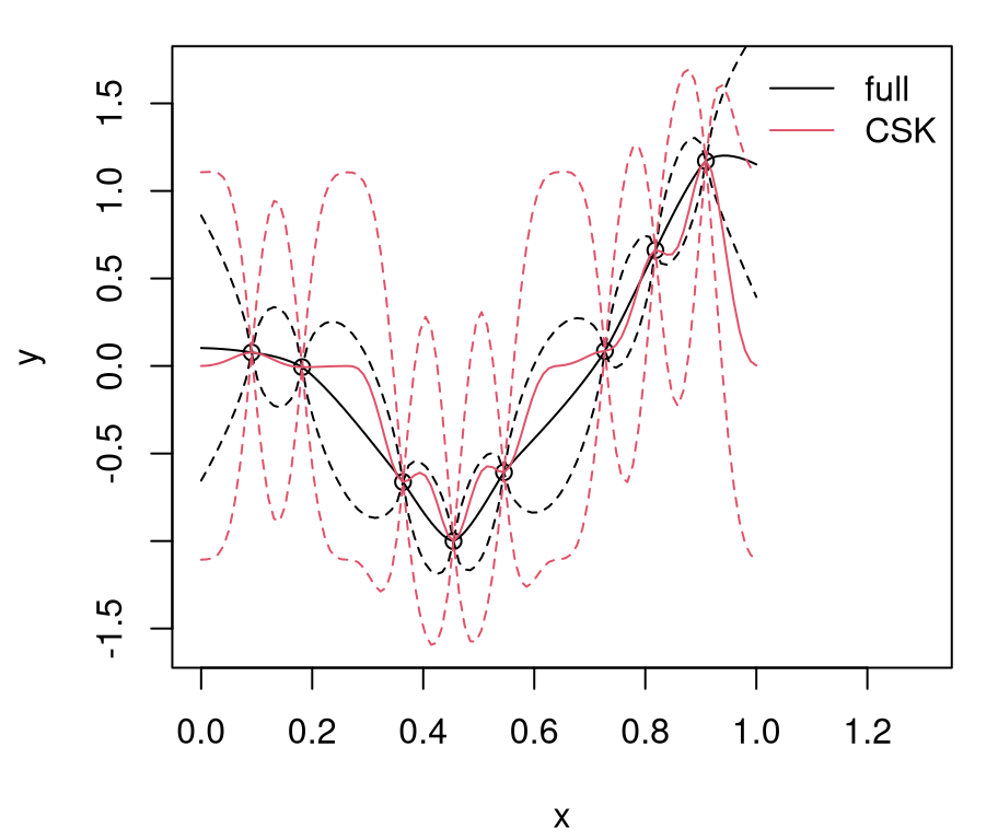
FIGURE 9.1: Predictions under CSK compared to the ideal full GP.
Relative to the ideal baseline, Bohman CSK predictions are too wiggly in the mean and too wide in terms of uncertainty. Predictive means are off because aggregation transpires in a narrower window. Variance is larger simply because sparse \(K\) leads to larger \(K^{-1}\). Evidently, inducing sparsity can have deleterious effects on GP prediction equations. What can be done?
9.1.2 Sharing load between mean and variance
A key idea in Kaufman et al. (2011) is to “mop up” long range non-linearity with rich mean structure, leaving a residual that may be modeled by shorter-range (sparse) correlations, via CSKs. In the GP surrogate modeling landscape, where mean-zero processes are the default, this represents somewhat of a paradigm shift. In ML and geostatistics, nonzero mean modeling is more common however simple linear means are the norm. Shifting more of the burden of modeling from covariance to mean is clever because it taps an underutilized resource. There are, of course, many ways that idea could be operationalized. Recall, e.g., that there are covariance kernels that can implement linear means (§5.3.3). Kaufman’s partition of focus, shifting between mean and variance, is therefore somewhat arbitrary. Yet human capacity to intuit statistical modeling dynamics generally favors locations over scales.
One alternative that’s similar to Kaufman’s idea in spirit, but different in form, is full-scale approximation [FSA; Sang and Huang (2012)]. FSA partitions effort between two spatial processes: a predictive process [PP; Banerjee et al. (2008); AO Finley et al. (2009)] for long range dependence, and a CSK for short-range spatial correlations. To establish a conceptual link between Kaufman and FSA, imagine the PP mapping to a nonparametric (nonlinear) mean structure. That analogy is imperfect because PPs are covariance-centric. Inference remains tractable because PPs emit a reduced rank approximation whose covariance structure can be decomposed quickly through the Sherman–Morrison–Woodbury identity, circumventing \(\mathcal{O}(n^3)\) matrix manipulation.
A downside to FSA is that implementing PP requires inferring a potentially large set of reference knots whose desired number, and subsequent inference, may become unwieldy as input dimension gets large. Many of the geo-spatial applications targeted by FSA/PP are two-dimensional, where they have enjoyed considerable success in large-\(n\) settings. While there are no fundamental or theoretical barriers to applying FSA more widely, e.g., to address larger input spaces more common in computer experiments and ML, I’m unaware of any successful ports to surrogate modeling. Pseudo inputs (Snelson and Ghahramani 2006), an ML take on PPs, have been applied more widely, but to my knowledge they have not been combined with CSK or an FSA-style analysis.
Kaufman’s rich-mean/CSK hybrid more squarely targets modestly higher-dimensional computer surrogate modeling contexts. For that reason, the narrative here focuses on that approach. You may recall from a homework problem in §5.5 that augmenting GPs with unknown linear mean structure can be accommodated analytically: closed-form expressions concentrate out – i.e., marginalize in the Bayesian setting, or replace with MLE for profile likelihoods – unknown regression coefficients, even ones derived from rather large nonlinear bases. The result is an inferential procedure demanding time in \(\mathcal{O}(n (n_{\mathrm{sparse}}^2) + p^3)\) where \(n_{\mathrm{sparse}}\) is the average number of nonzero entries in a row of a CSK matrix, and \(p\) is the size of the basis encoding the mean.
There are many reasonable families of bases to choose from. Kaufman et al. found that Legendre polynomials work well. The presentation below reverse engineers some of the computational details from their setup, which is packaged together in an R library called SparseEm (for sparse emulation) that can be downloaded from Cari Kaufman’s web page.
Unfortunately, Cari’s version fails to install in more modern R environments. I’ve provided a slightly modified version which is more up-to-date in terms of package structure, and should install for most Rs. Code below creates a degree four Legendre polynomial basis over training x values used by the simple 1d example in Figure 9.1.
leg01 <- legFun(0, 1)
degree <- 4
X <- leg01(x, terms=polySet(1, degree, 2, degree))
colnames(X) <- paste0("l", 0:(ncol(X) - 1))
X <- data.frame(X)
X
## l0 l1 l2 l3 l4
## 1 1 -1.4171 1.1273 -0.3757 -0.5243
## 2 1 -1.1022 0.2402 0.8210 -1.2784
## 3 1 -0.4724 -0.8686 0.9482 0.3608
## 4 1 -0.1575 -1.0903 0.3558 1.0329
## 5 1 0.1575 -1.0903 -0.3558 1.0329
## 6 1 0.7873 -0.4250 -1.1827 -0.6391
## 7 1 1.1022 0.2402 -0.8210 -1.2784
## 8 1 1.4171 1.1273 0.3757 -0.5243First, let’s see how well this basis works on its own, i.e., in a linear regression with iid noise structure (no GP). Notice that leg01 generates its own intercept column.
This leg01 basis must also be evaluated on the xx testing grid before it can be fed into predict.lm.
XX <- leg01(xx, terms=polySet(1, degree, 2, degree))
colnames(XX) <- paste0("l", 0:(ncol(X) - 1))
p <- predict(lfit, newdata=data.frame(XX), interval="prediction", level=0.9)
Figure 9.2 augments Figure 9.1. Perhaps with all those lines the plot is a bit busy. Yet it’s plain to see that the new leg01 fit, using lm on a Legendre basis, offers a better fit than CSK, but perhaps not as good as the ideal full GP fit.
plot(x, y, xlim=c(0, 1.35), ylim=range(q101, q201, p[,2], p[,3]))
lines(xx, m)
lines(xx, q1, lty=2)
lines(xx, q2, lty=2)
lines(xx, m01, col=2)
lines(xx, q101, col=2, lty=2)
lines(xx, q201, col=2, lty=2)
lines(xx, p[,1], col=3)
lines(xx, p[,2], col=3, lty=2)
lines(xx, p[,3], col=3, lty=2)
legend("topright", c("full", "CSK", "leg01"), lty=1, col=1:3, bty="n")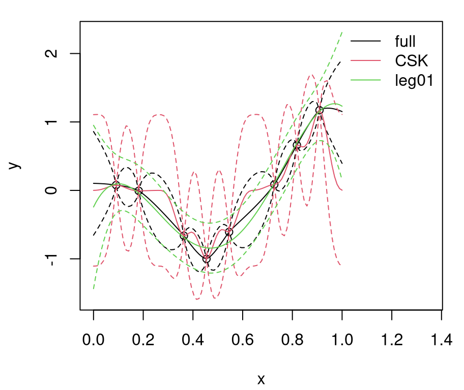
FIGURE 9.2: Legendre-basis linear prediction versus CSK and the ideal GP from Figure 9.1.
The linear/Legendre predictive surface is over-smooth, and consequently its error-bars are everywhere too large compared to ideal. Independent error modeling is a mismatch to our data generating mechanism, being used here to exemplify inherently deterministic computer model simulation. CSK’s error-bars can be even wider, but that surface still interpolates due to its nugget-free inverse distance-based covariance structure. It may be worth repeating this example in your own R session to observe a diversity of behaviors across data realizations and subsequent fits. You might also try higher degree Legendre bases (5 or 6, say).
Separately, neither Legendre basis nor CSK are on par with the ideal full GP, but how about together? As a quick illustration of potential, with a more coherent and Bayesian hybrid on the horizon, consider applying CSK on residuals from Legendre basis-derived fitted values.
m2 <- t(KX01) %*% Ki01 %*% lfit$resid
tau22 <- drop(t(lfit$resid) %*% Ki01 %*% lfit$resid)/n
Sigma2 <- tau22*(1 - t(KX01) %*% Ki01 %*% KX01)
Now consider predictive summaries formed by combining Legendre basis means with CSK covariances. Uncertainties are not properly managed in this hybrid, but my aim is simply to illustrate potential.
m2 <- p[,1] + m2
q12 <- qnorm(0.05, m2, sqrt(diag(Sigma2)))
q22 <- qnorm(0.95, m2, sqrt(diag(Sigma2)))
Figure 9.3 shows the resulting predictive surface. In place of green Legendre lines and red CSK lines, blue hybrid lines show how Legendre–CSK predictions compare to the ideal GP fit from earlier.
plot(x, y, xlim=c(0, 1.35), ylim=range(q1, q2, q12, q22))
lines(xx,m)
lines(xx, q1, lty=2)
lines(xx, q2, lty=2)
lines(xx, m2, col=4)
lines(xx, q12, col=4,lty=2)
lines(xx, q22, col=4,lty=2)
legend("topright", c("full", "hybrid"), lty=1, col=c(1,4), bty="n")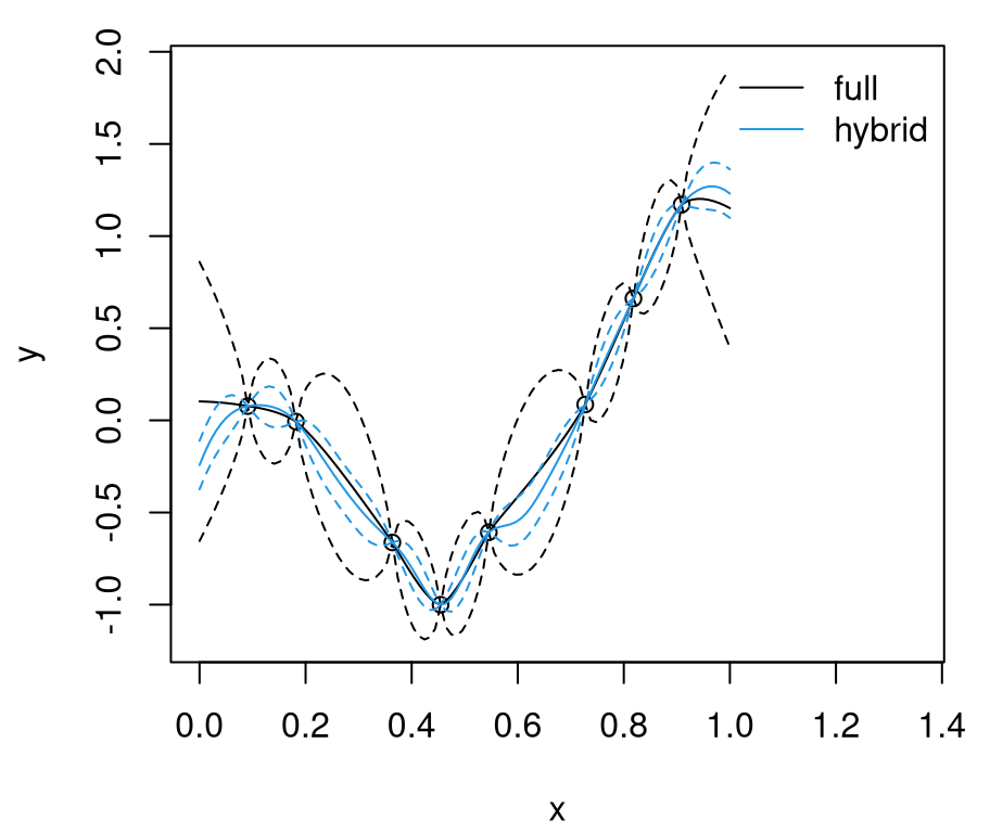
FIGURE 9.3: Comparing hybrid Legendre basis/CSK covariance to the ideal GP.
Although the two surfaces are not identical, they’re indeed very similar. Combining a Legendre basis-expanded linear mean with CSK structure on residuals does an excellent job of mimicking an ideal GP fit, at least on this very simple example. Observe that the hybrid predictive surface interpolates. It bears repeating that this illustration doesn’t provide full UQ. In particular, we used only the mean of the Legendre basis fit p[,1], ignoring uncertainty stored in p[,2:3]. So our fitted error-bars should actually be even wider. At the same time, we cheated by using true values of the correlation function in our ideal GP fit as plug-ins. So our benchmark is similarly too good to be true. Finally, we didn’t estimate the CSK range parameter \(r_{\max}\); the only hyperparameter fit from data was scale \(\hat{\tau}^2\) …
##    ideal CSKresid
## 0.452666 0.006399
… which is (reasonably) lower for the residual process, compared to the original.
9.1.3 Practical Bayesian inference and UQ
Kaufman et al. argue that the simplest, coherent way to put this hybrid together, and fully account for all relevant uncertainties in prediction while retaining a handle on trade-offs between computational complexity and accuracy (though CSK sparsity), is with Bayesian hierarchical modeling. They describe a prior linking together separable \(r_{\max,j}\) hyperparameters, for each input dimension \(j\). That prior encourages coordinates to trade-off against one another – competing in a manner not unlike in L1 penalization for linear regression using lasso – to produce a covariance matrix with a desired degree of sparsity. That is, some directions yield zero correlations faster than others as a function of coordinate-wise distance. Specifically, Kaufman et al. recommend
\[\begin{equation} r_{\max} \mbox{ uniform in } R_C = \left\{ r_{\max} \in \mathbb{R}^d : r_{\max,j} \geq 0, \; \sum_{j=1}^d r_{\max,j} \leq C \right\}. \tag{9.1} \end{equation}\]
Said another way, this penalty allows some \(r_{\max,j}\) to be large to reflect a high degree of correlation in particular input directions, shifting the burden of sparsity to other coordinates. Parameter \(C\) determines the level of sparsity in the resulting MVN correlation matrix.
That prior on \(r_{\max}\) is then paired with the usual reference priors for scale \(\tau^2\) and regression coefficients \(\beta\) through the Legendre basis. Conditional on \(r_{\max}\), calculations similar to those required for an exercise in §5.5, analytically integrating out \(\tau^2\) and \(\beta\), yield closed form expressions for the marginal posterior density. For details, see, e.g., Appendix A of Gramacy (2005). Inference for \(r_{\max}\) and any other kernel hyperparameters may then be carried out with a conventional mixture of Metropolis and Gibbs sampling steps.
It remains to choose a \(C\) yielding enough sparsity for tractable calculation given data sizes present in the problem on hand. Kaufman et al. produced a map, which I shall not duplicate here, relating degree of sparsity to computation time for various data sizes, \(n\). That map helps mitigate search efforts, modulo computing architecture nuances, toward identifying \(C\) yielding a specified degree of sparsity. Perhaps more practically, they further provide a numerical procedure which estimates the value of \(C\) required, after fixing all other choices for priors and their hyperparameters. I shall illustrate that pre-processing step momentarily.
As one final detail, Kaufman et al. recommend Legendre polynomials up to degree 5 in a “tensor product” form for their motivating cosmology example, including all main effects, and all two-variable interactions in which the sum of the maximum exponent in each interacting variable is constrained to be less than or equal to five. However, in their simpler coded benchmark example, which we shall borrow for our illustration below, it would appear they prefer degree 2.
Borehole example
Consider the borehole data, which is a classic synthetic computer simulation example (MD Morris, Mitchell, and Ylvisaker 1993), originally described by Worley (1987). It’s a function of eight inputs, modeling water flow through a borehole.
\[ y = \frac{2\pi T_u [H_u - H_l]}{\log\left(\frac{r}{r_w}\right) \left[1 + \frac{2 L T_u}{\log (r/r_w) r_w^2 K_w} + \frac{T_u}{T_l} \right]}. \]
Input ranges are
\[ \begin{aligned} r_w &\in [0.05, 0.15] & r &\in [100,50000] & T_u &\in [63070, 115600] \\ T_l &\in [63.1, 116] & H_u &\in [990, 1110] & H_l &\in [700, 820] \\ L &\in [1120, 1680] & K_w &\in [9855, 12045]. \end{aligned} \]
The function below provides an implementation in coded inputs.
borehole <- function(x)
 {
  rw <- x[1]*(0.15 - 0.05) + 0.05
  r <-  x[2]*(50000 - 100) + 100
  Tu <- x[3]*(115600 - 63070) + 63070
  Hu <- x[4]*(1110 - 990) + 990
  Tl <- x[5]*(116 - 63.1) + 63.1
  Hl <- x[6]*(820 - 700) + 700
  L <-  x[7]*(1680 - 1120) + 1120
  Kw <- x[8]*(12045 - 9855) + 9855
  m1 <- 2*pi*Tu*(Hu - Hl)
  m2 <- log(r/rw)
  m3 <- 1 + 2*L*Tu/(m2*rw^2*Kw) + Tu/Tl
  return(m1/m2/m3)
 }
Consider the following Latin hypercube sample (LHS; §4.1) training and testing partition a la Algorithm 4.1.
n <- 4000
nn <- 500
m <- 8
library(lhs)
x <- randomLHS(n + nn, m)
y <- apply(x, 1, borehole)
X <- x[1:n,]
Y <- y[1:n]
XX <- x[-(1:n),]
YY <- y[-(1:n)]
Observe that the problem here is bigger than any we’ve entertained so far in this text. However it’s worth noting that \(n=4000\) is not too big for conventional GPs. Following from Kaufman’s example, we shall provide a full GP below which (in being fully Bayesian and leveraging a Legendre basis-expanded mean) offers a commensurate look for the purpose of benchmarking computational demands. Yet Appendix A illustrates a thriftier GP implementation leveraging the MKL library which can handle more than \(n=10000\) training data points on this very same borehole problem. But that compares apples with oranges. Therefore we shall press on with the example, whose primary role – by the time the chapter is finished – will anyway be to serve as a straw man against more recent advances in the realm of local–global GP approximation.
The first step is to find the value of \(C\) that provides a desired level of sparsity. I chose 99% sparse through an argument den specifying density as the opposite of sparsity.
## [1] 2.708Next, R code below sets up a degree-two Legendre basis with all two-variable interactions, and then collects two thousand samples from the posterior. Compute time is saved for later comparison. Warnings that occasionally come from spam, when challenges arise in solving sparse linear systems, are suppressed in order to keep the document clean.
D <- I <- 2
B <- 2000
tic <- proc.time()[3]
suppressWarnings({
  samps99 <- mcmc.sparse(Y, X, mc=C, degree=D, maxint=I,
    B=B, verbose=FALSE)
})
time99 <- as.numeric(proc.time()[3] - tic)
Output samps99 is a B \(\times\) d matrix storing \(r_{\max,j}\) samples from the posterior distribution for each input coordinate, \(j=1,\dots,d\). Trace plots for these samples are shown in Figure 9.4. The left panel presents each \(r_{\max, j}\) marginally; on the right is their aggregate as in the definition of \(R_C\) (9.1). Observe how that aggregate bounces up against the estimated \(C\)-value of 2.71. Even with Legendre basis mopping up a degree of global nonlinearity, the posterior distribution over \(r_{\max, j}\) wants to be as dense as possible in order to capture spatial correlations at larger distances. A low \(C\)-value is forcing coordinates to trade off against one another in order to induce the desired degree of sparsity.
par(mfrow=c(1,2))
matplot(samps99, type="l", xlab="iter")
plot(rowSums(samps99), type="l", xlab="iter", ylab="Rc")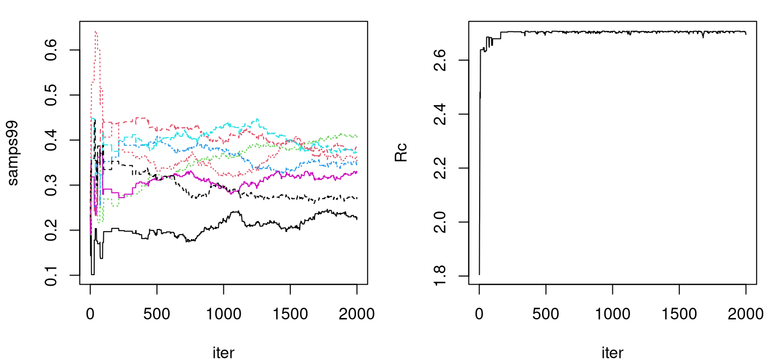
FIGURE 9.4: Trace plots of \(r_{\max,j}\) (left) and their aggregate \(\sum_j r_{\max, j}\) (right).
Both trace plots indicate convergence of the Markov chain after five hundred or so iterations followed by adequate – certainly not excellent – mixing. Marginal effective sample size calculations indicate that very few “equivalently independent” samples have been obtained from the posterior, however this could be improved with a longer chain.
## [1] 1.925 1.932 2.013 2.762 2.142 4.139 3.686 1.632Considering that it has already taken 46 minutes to gather these two thousand samples, it may not be worth spending more time to get a bigger collection for this simple example. (We’ll need even more time to convert those samples into predictions.)
## [1] 45.87Instead, perhaps let me encourage the curious reader to explore longer chains offline. Pushing on, the next step is to convert those hyperparameters into posterior predictive samples on a testing set. Below, discard the first five hundred iterations as burn-in, then save subsamples of predictive evaluations from every tenth iteration thereafter.
index <- seq(burnin+1, B, by=10)
tic <- proc.time()[3]
suppressWarnings({
  p99 <- pred.sparse(samps99[index,], X, Y, XX, degree=D,
    maxint=I, verbose=FALSE)
})
time99 <- as.numeric(time99 + proc.time()[3] - tic)
time99/60
## [1] 54.35The extra work required to make this conversion depends upon the density of the predictive grid, XX. In this particular case it doesn’t add substantially to the total compute time, which now totals 54 minutes. The keen reader will notice that we didn’t factor in time to calculate \(C\) with find.tau above. Relative to other calculations, this represents a rather small, fixed-cost pre-processing step.
Before assessing the quality of these predictions, consider a couple alternatives to compare to. Kaufman et al. provide a non-sparse version, that otherwise works identically, primarily for timing and accuracy comparisons. That way we’ll be comparing apples to apples, at least in terms of inferential apparatus, when it comes to computation time. Working with dense covariance matrices in this context is really slow. Therefore, the code below collects an order of magnitude fewer MCMC samples from the posterior. (Sampling and predictive stages are combined.) Again, I encourage the curious reader to gather more for a fairer comparison.
tic <- proc.time()[3]
suppressWarnings({
  samps0 <- mcmc.nonsparse(Y, X, B=B/3, verbose=FALSE)
})
index <- seq(burnin/3 + 1, B/3, by=10)
suppressWarnings({
  p0 <- pred.nonsparse(samps0[index,], X, Y, XX, 2, verbose=FALSE)
})
time0 <- as.numeric(proc.time()[3] - tic)
As illustrated in Figure 9.5, 667 samples are not nearly sufficient to be confident about convergence. Admittedly, I’m not sure why the mixing here seems so much worse than in the CSK analog. It may have been that Kaufman didn’t put as much effort into fine-tuning this straw man relative to their showcase methodology.
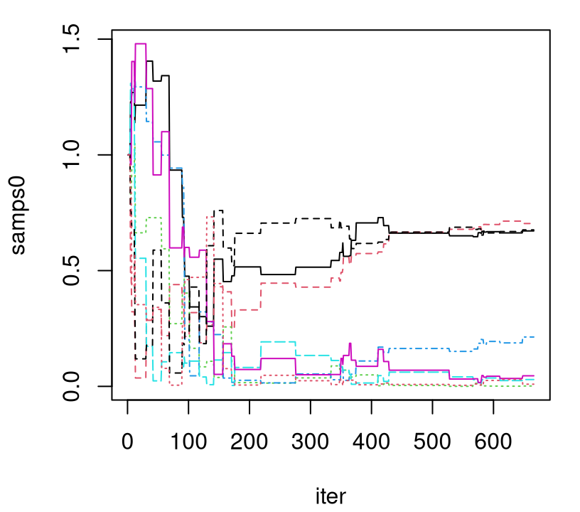
FIGURE 9.5: Trace plot of lengthscales under the full (non CSK) GP posterior; compare to the left panel of Figure 9.4.
Considering the amount of time it took to get as many samples as we did, we’ll have to be content with extrapolating a bit to make a proper timing comparison.
## [1] 51.75Gathering the same number of samples as in the 99% sparse CSK case would’ve required more than 2 hours of total compute time. For a comparison on accuracy grounds, consider pointwise proper scores via Eq. (27) from Gneiting and Raftery (2007). Also see §8.1.4. Higher scores are better.
scorep <- function(YY, mu, s2) { mean(-(mu - YY)^2/s2 - log(s2)) }
scores <- c(sparse99=scorep(YY, p99$mean, p99$var),
  dense=scorep(YY, p0$mean, p0$var))
scores
## sparse99 dense
## -1.918 -6.962CSK is both faster and more accurate on this example. It’s reasonable to speculate that the dense/ordinary GP results could be improved with better MCMC. Perhaps MCMC proposals, tuned to work well for short \(r_{\max,j}\) on residuals obtained from a rich Legendre basis, work rather less well for ordinary lengthscales \(\theta_j\) applied directly on the main process. In §9.3.4 we’ll show how a full GP under MLE hyperparameters can be quite accurate on these data.
To add one final comparator into the mix, let’s see how much faster and how much less accurate a 99.9% sparse version is. Essentially cutting and pasting from above …
C <- find.tau(den=1 - 0.999, dim=ncol(x))*ncol(x)
tic <- proc.time()[3]
suppressWarnings({
  samps999 <- mcmc.sparse(Y, X, mc=C, degree=D, maxint=I,
    B=B, verbose=FALSE)
})
index <- seq(burnin+1, B, by=10)
suppressWarnings({
  p999 <- pred.sparse(samps999[index,], X, Y, XX, degree=D,
    maxint=I, verbose=FALSE)
})
time999 <- as.numeric(proc.time()[3] - tic)
In terms of computing time, the 99.9% sparse version is almost an order of magnitude faster.
##  sparse99     dense sparse999
##    3260.9    3104.9     404.8
In terms of accuracy, it’s just a little bit worse than the 99% analog and much better than the slow and poorly mixing full GP.
##  sparse99     dense sparse999
##    -1.918    -6.962    -2.105
To summarize this segment on CSKs, consider the following notes. Sparse covariance matrices decompose faster compared to their dense analogs, but the gap in execution time is only impressive when matrices are very sparse. In that context, intervention is essential to mop up long-range structure left unattended by all those zeros. A solution entails hybridization between processes targeting long- and short-distance correlation. Kaufman et al. utilize a rich mean structure; Sang and Huang’s FSA stays covariance-centric. Either way, both agree that Bayesian posterior sampling is essential to average over competing explanations. We have seen that the MCMC required can be cumbersome: long chains “eat up” computational savings offered by sparsity. Nevertheless, both camps offer dramatic success stories. For example, Kaufman fit a surrogate to more than twenty thousand runs of a photometric redshift simulation – a cosmology example – in four input dimensions, and predict with full UQ at more then eighty thousand sites. Results are highly accurate, and computation time is reasonable.
One big downside to these ideas, at least in the context of our motivation for this chapter, is that neither approach addresses nonstationarity head on. Computational demands are eased, somewhat, but modeling fidelity has not been substantially increased. I qualify with “substantially” because the introduction of a basis-expanded mean does hold the potential to enhance even though it was conceived to compensate. Polynomial bases, when dramatically expanded both by location and degree, do offer a degree of nonstationary flexibility. Smoothing splines are a perfect example; also see the splines supplement. But such techniques break down computationally when input dimension is greater than two. Exponentially many more knots are required as input dimension grows. A more deliberate and nonparametric approach to obtaining local variation in a global landscape could represent an attractive alternative.
9.2 Partition models and regression trees
Another way to induce sparsity in the covariance structure is to partition the input space into independent regions, and fit separate surrogates therein. The resulting covariance matrix is block-diagonal after row–column reordering. In fact, you might say it’s implicitly block-diagonal because it’d be foolish to actually build such a matrix. In fact, even “thinking” about the covariance structure on a global scale, after partitioning into multiple local models, can be a hindrance to efficient inference and effective implementation.
The trouble is, it’s hard to know just how to split things up. Divide-and-conquer is almost always an effective strategy computationally. But dividing haphazardly can make conquering hard. When statistical modeling, it’s often sensible to let the data decide. Once we’ve figured that out – i.e., how to let data say how it “wants” to be partitioned for independent modeling – many inferential and computational details naturally suggest themselves.
One happy consequence of partitioning, especially when splitting is spatial in nature, is a cheap nonstationary modeling mechanism. Independent latent processes and hyperparameterizations, thinking particularly about fitting GP surrogates to each partition element, kills two birds with one stone: 1) disparate spatial dynamics across the input space; 2) smaller matrices to decompose for faster local inference and prediction. The downside is that all bets for continuity are off. That “bug” could be a “feature”, e.g., if the data generating mechanism is inherently discontinuous, which is not as uncommon as you might think. But more often a scheme for smoothing, or averaging over all (likely) partitions is desired.
Easy to say, hard to do. I know of only two successful attempts involving GPs on partition elements: 1) with Voronoi tessellations (Kim, Mallick, and Holmes 2005); 2) with trees (Gramacy and Lee 2008a). In both cases, those references point to the original attempts. Other teams of authors have subsequently refined and extended these ideas, but the underlying themes remain the same. Software is a whole different ballgame; I know of only one package for R.
Tessellations are easy to characterize mathematically, but a nightmare computationally. Trees are easy mathematically too, and much friendlier in implementation. Although no walk in the park, tree data structures are well developed from a software engineering perspective. Translating tree data structures from their home world of computer science textbooks over to statistical modeling is relatively straightforward, but as always the devil is in the details.
Figure 9.6 shows a partition tree \(\mathcal{T}\) in two views. The left-hand drawing offers a graph view, illustrating a tree with two internal, or splitting nodes, and three leaf or terminal nodes without splits. Internal nodes are endowed with splitting criteria, which in this case refers to conditional splits in a two-dimensional \(x\)-space. Internal nodes have two children, called siblings. All nodes have a parent except the root, paradoxically situated at the top of the tree.
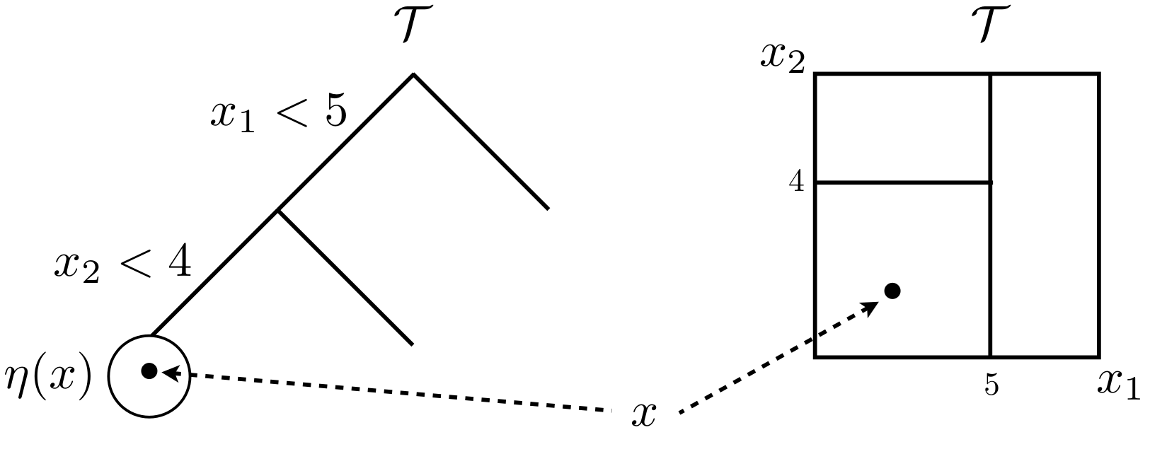
FIGURE 9.6: Tree graph (left) and partition of a 2d input space (right). Borrowed from H. Chipman et al. (2013) with many similar variations elsewhere; used with permission from Wiley.
The right-hand drawing illustrates the recursive nature of those splits geographically in the input space, creating an axis-aligned partition. A generic 2d input coordinate \(x\) would land in one of the three leaf nodes, depending on the setting of its two coordinates \(x_1\) and \(x_2\). Leaf node \(\eta(x)\) resides in the lower-left partition of the input space.
For statistical modeling, the idea is that recursive, axis-aligned, splits represent a simple yet effective way to divvy up the input space \(\mathcal{X}\) into independent predictive models for responses \(y\). Predictions \(\hat{y}(x)\) are dictated by tree structure, \(\mathcal{X}\) and leaf model: historically, a simple prediction rule tailored to the subset of data residing at each terminal node. My plan is to showcase GPs at the leaves, but let’s take a step back first.
9.2.1 Divide-and-conquer regression
Use of trees in regression dates back to AID (automatic interaction detection) by Morgan and Sonquist (1963). Classification and regression trees [CART; Breiman et al. (1984)], a suite of methods obtaining fitted partition trees, popularized the idea. The selling point was that trees facilitate parsimonious divide-and-conquer, leading to flexible yet interpretable modeling.
Fitting partition structure (depth, splits, etc.) isn’t easy, however. You need a leaf model/prediction rule, goodness-of-fit criteria, and a search algorithm. And there are lots of very good ways to make choices in that arena. In case it isn’t yet obvious, I prefer likelihood whenever possible. Although other approaches are perhaps more common in the trees literature, with as many/possibly more contributions from computer science as statistics, likelihoods rule the roost as a default in modern statistics.
Given a particular tree, \(\mathcal{T}\), the (marginal) likelihood factorizes into a product form.
\[ p(y^n \mid \mathcal{T}, x^n) \equiv p(y_1, \dots, y_n \mid \mathcal{T}, x_1,\dots, x_n) = \prod_{\eta \in \mathcal{L}_{\mathcal{T}}} p(y^\eta \mid x^\eta) \]
Above, shorthand \(x^n = x_1,\dots,x_n\) and \(y^n = y_1, \dots, y_n\) represents the full dataset of \(n\) pairs \((x,y)^n = \{(x_i, y_i):\; i=1,\dots,n\}\). Analogously, superscript \(\eta\) represents those elements of the data which fall into leaf node \(\eta\). That is, \((x,y)^\eta = \{(x_i, y_i):\; x_i\in \eta, \; i=1,\dots,n\}\). The product arises from independent modeling, and by indexing over all leaf nodes in \(\mathcal{T}\), \(\eta \in \mathcal{L}_{\mathcal{T}}\), we cover all indices \(i \in \{1,\dots,n\}\). All that remains in order to complete the specification is to choose a model for \(p(y^\eta \mid x^\eta)\) to apply at leaf nodes \(\eta\).
Usually such models are specified parametrically, via \(\theta_\eta\), but calculations are simplified substantially if those parameters can be integrated out. Hence the parenthetical “marginal” above. The simplest leaf model for regression is the constant model with unknown mean and variance \(\theta_\eta = (\mu_\eta, \sigma^2_\eta)\):
\[ \begin{aligned} p(y^\eta \mid \mu_\eta, \sigma^2_\eta, x^\eta) &\propto \sigma_\eta^{-|\eta|} \exp\left\{\textstyle-\frac{1}{2\sigma_\eta^2} \sum_{y \in \eta} (y - \mu_\eta)^2\right\} \\ \mbox{so that } \;\; p(y^\eta \mid x^\eta) & = \frac{1}{(2\pi)^{\frac{|\eta|-1}{2}}}\frac{1}{\sqrt{|\eta|}} \left(\frac{s_\eta^2}{2}\right)^{-\frac{|\eta|-1}{2}} \Gamma\left(\frac{|\eta|-1}{2}\right) \end{aligned} \]
upon taking reference prior \(p(\mu_\eta, \sigma_\eta^2) \propto \sigma_\eta^{-2}\). Above, \(|\eta|\) is a count of the number of data points in leaf node \(\eta\), and \(s_\eta^2 \equiv \hat{\sigma}_\eta^2\) is the typical residual sum of squares from \(\bar{y}_\eta \equiv \hat{\mu}_\eta\). Concentrated analogs, i.e., not committing to a Bayesian approach, are similar. However the Bayesian view is natural from the perspective of coherent regularization.
Clearly some kind of penalty on complexity is needed for inference, otherwise marginal likelihood is maximized when there’s one leaf for each observation. The original CART family of methods relied on minimum leaf-size and other heuristics, paired with a cross validation (CV) pruning stage commencing after greedily growing a deep tree. The fully Bayesian approach, which is more recent, has a more natural feel to it although at the expense of greater computation through MCMC. A silver lining, however, is that the Monte Carlo can smooth over hard breaks and lend a degree of continuity to an inherently “jumpy” predictive surface.
Completing the Bayesian specification requires a prior over trees, \(p(\mathcal{T})\). There were two papers, published at almost the same time, proposing a so-called Bayesian CART model, or what is known as the Bayesian treed constant model in the regression (as opposed to classification) context. Denison, Mallick, and Smith (1998) were looking for a light touch, and put a Poisson on the number of leaves, but otherwise specified a uniform prior over other aspects such as tree depth. H. A. Chipman, George, and McCulloch (1998) called for a more intricate class of priors which allowed heavier regularization to be placed on tree depth. Time says they won the argument, although the reasons for that are complicated. Almost everyone has since adopted the so-called CGM prior, although that’s not evidence of much except popularity. (VHS beat out BetaMax in the videotape format war, but not because the former is better.) If the last twenty years have taught us nothing, we’ve at least learned that a hearty dose of regularization – even when not strictly essential – is often a good default.
CGM’s prior is based on the following tree growing stochastic process. A tree \(\mathcal{T}\) may grow from one of its leaf nodes \(\eta\), which might be the root, with a probability that depends on the depth \(D_\eta\) of that node in the tree. The family of probabilities preferred by CGM, dictating terms for when such a leaf node might split into two new children, is provided by the expression below.
\[ p_{\mathrm{split}}(\eta,\mathcal{T}) = \alpha(1+D_{\eta})^{-\beta} \]
One can use this probability to simulate the tree growing process, generating recursively starting from a null, single leaf/root tree, and stopping when all leaves refuse to draw a split. CGM studied this distribution under various choices of hyperparameters \(0 < \alpha < 1\) and \(\beta \geq 0\) in order to provide insight into characteristics of trees which are typical under this prior.
Of course, the primary aim here isn’t to generate trees a priori, but to learn trees via partitions of the data and the subsequent patchwork of regressions they imply. For that, a density on \(\mathcal{T}\) is required. It’s simple to show that this prior process induces a prior density for tree \(\mathcal{T}\) through the probability that internal nodes \(\mathcal{I}_{\mathcal{T}}\) split and leaves \(\mathcal{L}_{\mathcal{T}}\) do not:
\[ p(\mathcal{T}) \propto \prod_{\eta\,\in\,\mathcal{I}_{\mathcal{T}}} p_{\mathrm{split}}(\eta, \mathcal{T}) \prod_{\eta\,\in\,\mathcal{L}_{\mathcal{T}}} [1-p_{\mathrm{split}}(\eta, \mathcal{T})]. \]
As in the DMS prior (Denison, Mallick, and Smith 1998), CGM retains uniformity on everything else: splitting location/dimension, number of leaf node observations. Note that a minimum number of observations must be enforced in order to ensure proper posteriors at the leaves. That is, under the reference prior \(p(\mu_\eta, \sigma_\eta^2) \propto \sigma_\eta^{-2}\), we must have at least \(|\eta| \geq 2\) observations in each leaf node \(\eta \in \mathcal{L}_{\mathcal{T}}\).
Inference
Posterior inference proceeds by MCMC. Note that there are no parameters except tree \(\mathcal{T}\) when leaf-node \(\theta_\eta\) are integrated out. Here is how a single iteration of MCMC would go. Randomly choose one of a limited number of stochastic tree modification operations (grow, prune, change, swap, rotate; more below), and conditional on that choice, randomly select a node \(\eta \in \mathcal{T}\) on which that proposed modification would apply. Those two choices comprise proposal \(q(\mathcal{T}, \mathcal{T}')\) for generating a new tree \(\mathcal{T}'\) from \(\mathcal{T}\), taking a step along a random walk in tree space. Accept the move with Metropolis–Hastings (MH) probability:
\[ \frac{p(\mathcal{T}' \mid y^n, x^n)}{p(\mathcal{T} \mid y^n, x^n)} \times \frac{q(\mathcal{T}', \mathcal{T})}{q(\mathcal{T}, \mathcal{T}')} = \frac{p(y^n \mid \mathcal{T}', x^n)}{p(y^n \mid \mathcal{T}, x^n)} \times \frac{p(\mathcal{T}')}{p(\mathcal{T})} \times \frac{q(\mathcal{T}', \mathcal{T})}{q(\mathcal{T}, \mathcal{T}')}. \]
There’s substantial scope for computational savings here with local moves \(q(\mathcal{T}, \mathcal{T}')\) in tree space, since many terms in the big product over \(\eta \in \mathcal{L}_{\mathcal{T}}\) in the denominator marginal likelihood, and over \(\eta' \in \mathcal{L}_{\mathcal{T'}}\) in the numerator one, would cancel for unaltered leaves in \(\mathcal{T} \rightarrow \mathcal{T}'\).
What do tree proposals \(q\) look like? Well, they can be whatever you like so long as they’re reversible, which is required by the ergodic theorem for MCMC convergence, providing samples from the target distribution \(p(\mathcal{T} \mid y^n, x^n)\). That basically means proposals must be matched with an opposite, undo proposal. Figure 9.7 provides an example of the four most popular tree moves, converting tree \(\mathcal{T}\) from Figure 9.6 to \(\mathcal{T}'\) shown in the same two views.
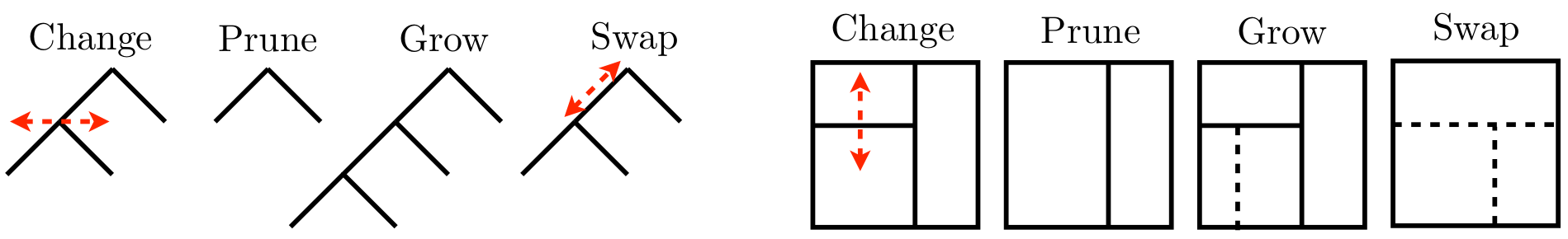
FIGURE 9.7: Random-walk proposals in tree space graphically (left four) and as partitions (right four). Borrowed from H. Chipman et al. (2013) with many similar variations elsewhere; used with permission from Wiley.
Observe that these moves have reversibility built in. Grow and prune are the undo of one another, and change and swap are the undo of themselves. Grow and prune are extremely local moves, acting only on leaf nodes and parents thereof, respectively. Swap and change are slightly more global as they may be performed on any internal node, or adjacent pair of nodes, respectively. Consequently, they may shuffle the contents of all their descendant leaves. Such “high up” proposals can have low MH acceptance rates because they tend to create \(\mathcal{T}'\) far from \(\mathcal{T}\).
Several new moves have been introduced to help. Gramacy and Lee (2008a) provide rotate which, like swap, acts on pairs of nodes which might reside anywhere in the tree. However, no matter how high up a rotation is, leaf nodes always remain unchanged. Thus acceptance is determined only by the prior. The idea comes from tree re-balancing in the computer science literature, for example as applied for red–black trees. Y. Wu, Tjelmeland, and West (2007) provide a radical restructure move targeting similar features, but with greater ambition. M. T. Pratola (2016) offers an alternative rotate targeting local moves which traverse disparate regions of partition space along contours of high, rather than identical likelihood.
To illustrate inference under the conventional move set, consider the motorcycle accident data in the MASS library for R. These data are derived from simulation of the acceleration of the helmet of a motorcycle rider before and after an impact. The pre- and post-whiplash effect, which we shall visualize momentarily, is extremely hard to model, whether using parametric (linear) models, or with GPs.
We shall utilize a Bayesian CART (BCART) implementation from the tgp package (Gramacy and Taddy 2016) on CRAN. One quirk of tgp is that you must provide a predictive grid, XX below, at the time of fitting. Trees are complicated data structures, which makes saving samples from lots of MCMC iterations cumbersome. It’s far easier to save predictions derived from those trees, obtained by dropping elements of \(x \in \mathcal{X} \equiv\) XX down to leaf(s). In fact, it’s sufficient to save the average means and quantiles accumulated over MCMC iterations. For each \(x \in \mathcal{X}\), one can separately aggregate \(\hat{\mu}_{\eta(x)}\) and quantiles \(\hat{\mu}_{\eta(x)} \pm 1.96\hat{\sigma}_{\eta(x)}\) for all \(\eta(x) \in \mathcal{L}_{\mathcal{T}}\), for every tree \(\mathcal{T}\) visited by the Markov chain, normalizing at the end. That quick description is close to what tgp does by default.
XX <- seq(0, max(mcycle[,1]), length=1000)
out.bcart <- bcart(X=mcycle[,1], Z=mcycle[,2], XX=XX, R=100, verb=0)
Another peculiarity here is the argument R=100, which calls for one hundred restarts of the MCMC. CGM observed that mixing in tree space can be poor, resulting in chains becoming stuck in local posterior maxima. Multiple restarts can help alleviate this. Whereas posterior mean predictive surfaces require accumulating predictive draws over MCMC iterations, the most probable predictions can be extracted after the fact. Code below utilizes predict.tgp to extract the predictive surface from the most probable tree, i.e., the maximum a posteriori (MAP) tree \(\hat{\mathcal{T}}\).
It’s worth reiterating that this way of working is different from the typical fit-then-predict scheme in R. The main prediction vehicle in tgp is driven by providing XX to bcart and similar methods. Still both surfaces, posterior mean and MAP, offer instructive visualizations. To that end, the R code below establishes a macro that I shall reuse, in several variations, to visualize predictive output from fitted tree models.
plot.moto <- function(out, outp)
 {
  plot(outp$XX[,1], outp$ZZ.km, ylab="accel", xlab="time",
    ylim=c(-150, 80), lty=2, col=1, type="l")
  points(mcycle)
  lines(outp$XX[,1], outp$ZZ.km + 1.96*sqrt(outp$ZZ.ks2), col=2, lty=2)
  lines(outp$XX[,1], outp$ZZ.km - 1.96*sqrt(outp$ZZ.ks2), col=2, lty=2)
  lines(out$XX[,1], out$ZZ.mean, col=1, lwd=2)
  lines(out$XX[,1], out$ZZ.q1, col=2, lwd=2)
  lines(out$XX[,1], out$ZZ.q2, col=2, lwd=2)
 }
Observe in the macro that solid bold (lwd=2) lines are used to indicate posterior mean predictive; thinner dashed lines (lty=2) indicate the MAP. On both, black (col=1) shows the center (mean of means or MAP mean) and red (col=2) shows 95% quantiles. Figure 9.8 uses this macro for the first time in the context of our Bayesian CART fit, also for the first time showing the training data.
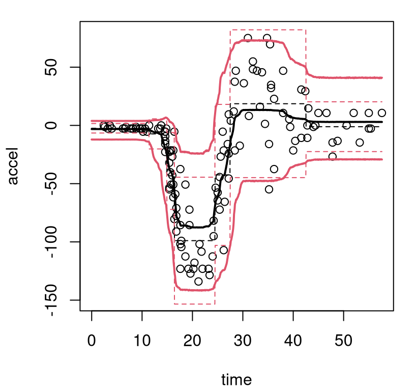
FIGURE 9.8: Bayesian treed constant model fit to the motorcycle accident data in terms of means and 95% quantiles. Posterior means are indicated by solid lines; MAP dashed.
What can be seen in these surfaces? Organic nonstationarity and heteroskedasticity, that’s what. The rate of change of outputs is changing as a function of inputs, and so is the noise level. Training data exhibit these features, and predictive surfaces are coping well, albeit not gracefully. Variances, exhibited by quantiles, may be too high (wide) at the end. The whiplash effect in the middle of the data appears overly dampened by forecasts on the testing grid.
The MAP surface (dashed lines) in the figure exemplifies an “old CART way” of regression. Hard breaks abound, being both unsightly and a poor surrogate for what are likely smooth physical dynamics. Posterior mean predictive summaries (solid lines) are somewhat more smooth. Averaging over the posterior for \(\mathcal{T}\) with MCMC smooths over abrupt transitions that come in disparate form with each individual sample from the chain. Yet the surface, even after aggregation, is still blocky: like a meandering staircase with rounded edges. A longer MCMC chain, or more restarts, could smooth things out more, but with diminishing return.
Other leaf models
One of the cool things about this setup is that any data type/leaf model may be used without extra computational effort if \(p(y^\eta \mid x^\eta)\) is analytic; that is, as long as we can evaluate the marginal likelihood, integrating out parameters \(\theta_\eta\) in closed form. Fully conjugate, scale-invariant, default (non-informative) priors on \(\theta_\eta\) make this possible for a wide class of models for response \(y\), even conditional on \(x\). A so-called Bayesian treed linear model [BTLM; HA Chipman, George, and McCulloch (2002)] uses
\[ \begin{aligned} p(y^\eta \mid \beta_\eta, \sigma_\eta^2, x^\eta) & \propto \sigma_\eta^{-|\eta|} \exp \{ (y^\eta - \bar{X}_\eta \beta_\eta)^2/2\sigma_\eta^2\} \quad \mbox{ and } \quad p(\beta_\eta, \sigma_\eta^2) \propto \sigma_\eta^{-2}. \end{aligned} \]
In that case we have
\[ p(y^\eta \mid x^{\eta}) = \frac{1}{(2\pi)^{\frac{|\eta|-d-1}{2}}} \left(\frac{|\mathcal{G}_\eta^{-1}|}{|\eta|}\right)^{\frac{1}{2}} \left(\frac{s_\eta^2-\mathcal{R}_\eta}{2}\right)^{-\frac{|\eta|-m-1}{2}} \Gamma\left(\frac{|\eta|-d-1}{2}\right), \]
where \(\mathcal{G}_\eta = \bar{X}_\eta^\top\bar{X}_\eta\), \(\mathcal{R}_\eta = \hat{\beta}_\eta^\top \mathcal{G}_\eta \hat{\beta}_\eta\) and intercept-adjusted \((m+1)\)-column \(\bar{X}_\eta\) is a centered design matrix derived from \(x^\eta\).
Without getting too bogged down in details, how about a showcase of BTLM in action through its tgp implementation? Again, we must specify XX during the fitting stage for full posterior averaging in prediction.
out.btlm <- btlm(X=mcycle[,1], Z=mcycle[,2], XX=XX, R=100, verb=0)
outp.btlm <- predict(out.btlm, XX=XX)
As before, a MAP predictor may be extracted after the fact. Figure 9.9 reuses the plotting macro in order to view the result, and qualitatively compare to the earlier BCART fit.
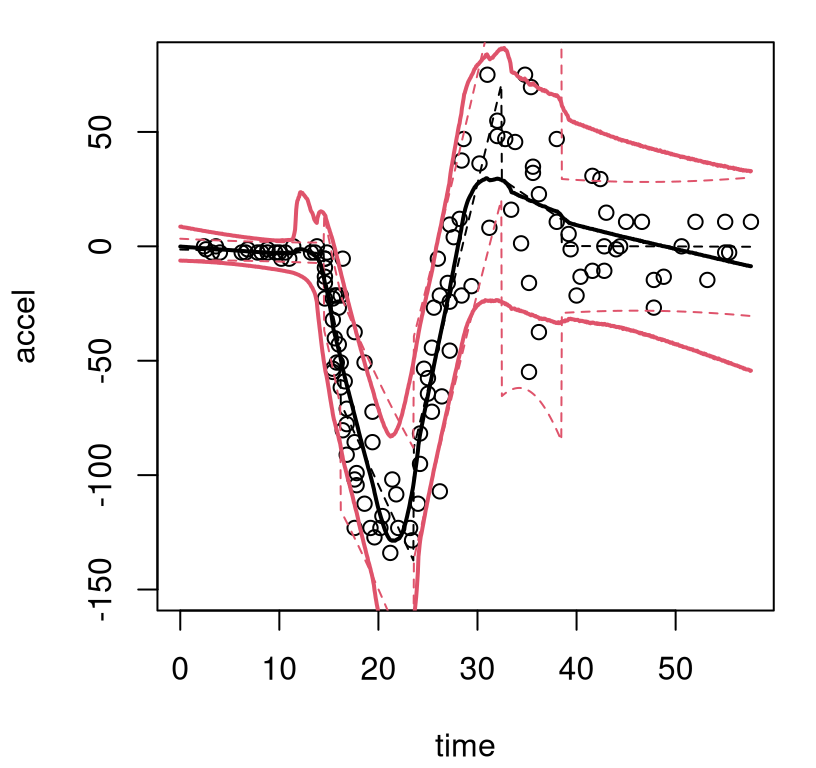
FIGURE 9.9: Bayesian treed linear model fit to the motorcycle accident data; compare to Figure 9.8.
The MAP surface (dashed) indicates fewer partitions compared to the BCART analog, but the full posterior average (solid) implies greater diversity in trees and linear-leaves over MCMC iterations. In particular, there’s substantial posterior uncertainty in timing of the impact, when acceleration transitions from level at zero into whiplash around time=14. For the right third of inputs there’s disagreement about both slope and noise level. Both BTLM surfaces, MAP and posterior mean, dampen the whiplash to a lesser extent compared to BCART. Which surface is better likely depends upon intended use.
If responses \(y\) are categorical, then a multinomial leaf model and Dirichlet prior pair leads to an analytic marginal likelihood (H. A. Chipman, George, and McCulloch 1998). Other members of the exponential family proceed similarly: Poisson, exponential, negative binomial… Yet to my knowledge none of these choices – besides multinomial – have actually been implemented in software as leaf models in a Bayesian setting.
Technically, any leaf model can be deployed by extending the MCMC to integrate over leaf parameters \(\theta_\eta\) too; in other words, replace analytic integration to calculate marginal likelihoods, in closed form, with a numerical alternative. Since the dimension of the parameter space is changing when trees grow or prune, reversible jump MCMC (Richardson and Green 1997) is required. Beyond that technical detail, a more practical issue is that deep trees/many leaves can result in a prohibitively large parameter space. An important exception is GPs. GPs offer a parsimonious take on nonlinear nonparametric regression, mopping up much of the variability left to the tree with simpler leaf models. GP leaves encourage shallow trees with fewer leaf nodes. At the same time, treed partitioning enables (axis aligned) regime changes in mean stationarity and skedasticity.
Before getting into further detail, let’s look at a stationary GP fit to the motorcycle data. The tgp package provides a Bayesian GP fitting method that works similarly to bcart and btlm. Since GP MCMC mixes well, fewer restarts need be entertained. (Even the default of R=1 works well.)
Although the code above executes an order of magnitude fewer MCMC iterations, runtimes (not quoted here) are much slower for BGP due to the requisite matrix decompositions. Figure 9.10, again using our macro, shows predictive surfaces which result.
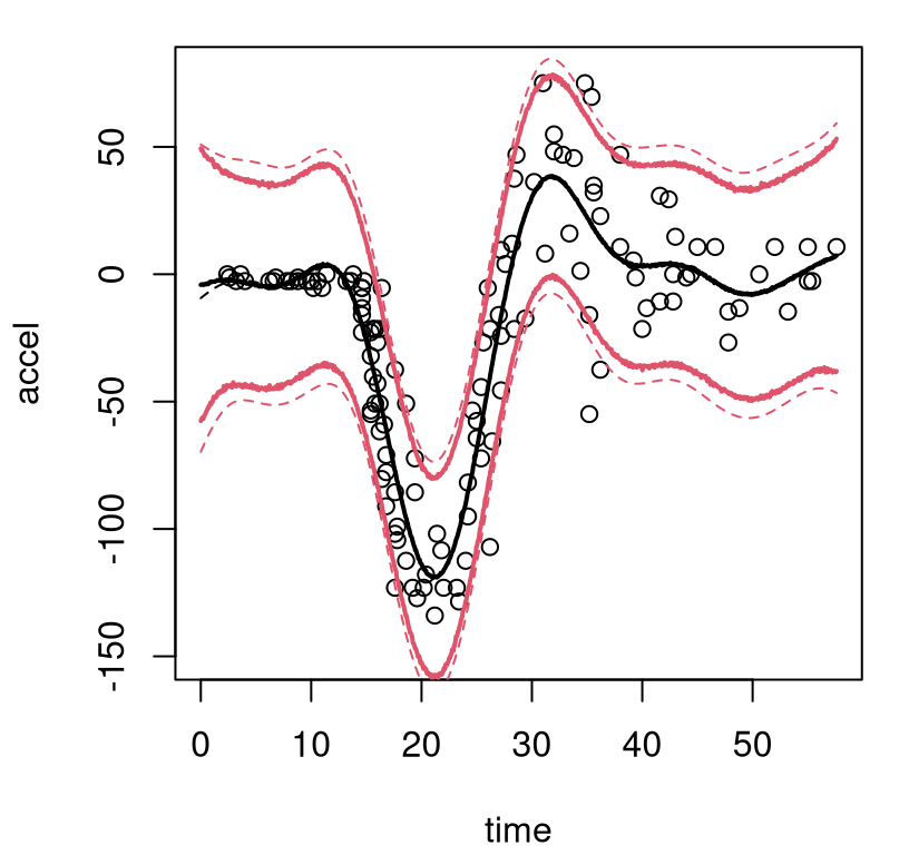
Both are nice and smooth, but lead to a less than ideal fit especially as regards variance. In fact you might say that GP and tree-based predictors are complementary. Where one is good the other is bad. Can they work together in harmony?
9.2.2 Treed Gaussian process
Bayesian treed Gaussian process (TGP) models (Gramacy and Lee 2008a) can offer the best of both worlds, marrying the smooth global perspective of an infinite basis expansion, via GPs, with the thrifty local adaptivity of trees. Their divide-and-conquer nature means faster computation from smaller matrix decompositions, and nonstationary and heteroskedasticity effects as conditionally independent leaves allow for disparate spatial dependencies. Perversely, the two go hand in hand. The more the training data exhibit nonstationary/heteroskedastic features, the more treed partitioning and the faster it goes!
There are too many modeling and implementation details to introduce here. References shall be provided – in addition to the original methodology paper cited above – in due course. For now the goal is to illustrate potential and then move on to more ambitious enterprises with TGP. The program is the same as above, using tgp from CRAN, but with btgp instead. Bayesian posterior sampling is extended to cover GP hyperparameters (lengthscales and nuggets) at the leaves.
Previous calls to tgp’s suite of b* functions specified verb=0 to suppress MCMC progress output printed to the screen by default. The call above is no exception. That output was suppressed because it was either excessive (bcart and btlm) or boring (bgp). Situated in-between on the modeling landscape, btgp progress statements are rather more informative, and less excessive, providing information about accepted tree moves and giving an online indication of trade-offs navigated between smooth and abrupt dynamics. I recommend trying verb=1.
Argument bprior="b0", above, is optional. By default, tgp fits a linear mean GP at the leaves, unless meanfn="constant" is given. Specifying bprior="b0" creates a hierarchical prior linking \(\beta_\eta\) and \(\sigma^2_\eta\), for all \(\eta \in \mathcal{L}_{\mathcal{T}}\), together. That makes sense for the motorcycle data because it starts and ends flat. Under the default setting of bprior="bflat", \(\beta_\eta\) and \(\sigma_\eta^2\) parameters of the linear mean are unrestricted. Results are not much different in that case.
As before, the MAP predictor may be extracted for comparison.
Figure 9.10, generated with our macro, provides a summary of both mean and MAP predictive surfaces.
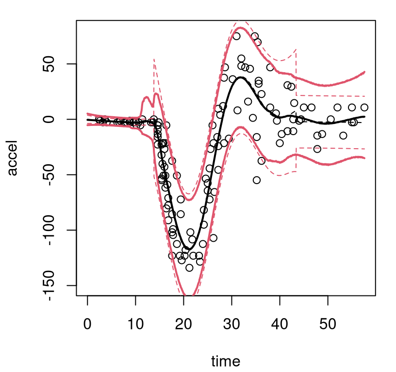
It’s hard to imagine a better compromise. Both surfaces offer excellent fits on their own, but the posterior mean clearly enjoys greater smoothness, which is warranted by the physics under study. Both surfaces, but particularly the posterior mean, reflect uncertainty in the location of the transition between zero-acceleration and whiplash dynamics for time \(\in (10,15)\). The posterior over trees supports many transition points in that region more-or-less equally.
Often having a GP at all leaves is overkill, and this is the case with the motorcycle accident data. The response is flat for the first third of inputs, and potentially flat in the last third too. Sometimes spatial correlation is only expressed in some input coordinates; linear may be sufficient in others. Gramacy and Lee (2008b) explain how a limiting linear model (LLM) can allow the data to determine the flexibility of the leaf model, offering a more parsimonious fit and speed enhancements when training data determine that a linear model is sufficient to explain local dynamics.
For now, consider how LLMs work in the simple 1d case offered by mcycle.
out.btgpllm <- btgpllm(X=mcycle[,1], Z=mcycle[,2], XX=XX, R=30,
  bprior="b0", verb=0)
outp.btgpllm <- predict(out.btgpllm, XX=XX)
Figure 9.12, showcasing btgpllm, offers a subtle contrast to the btgp fit shown in Figure 9.11.
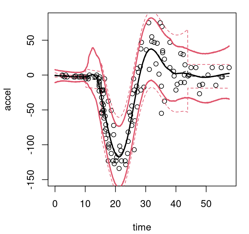
FIGURE 9.12: Bayesian treed GP with jumps to the limiting linear model (LLM) on the motorcycle data; compare to Figure 9.11.
Observe how the latter third of inputs enjoys a slightly tighter predictive interval in this setting, borrowing strength from the obviously linear (actually completely flat) fit to the first third of inputs. Transition uncertainty from zero-to-whiplash is also somewhat diminished.
For a two-dimensional example, revisit the exponential data first introduced in §5.1.2. In fact, that data was created to showcase subtle nonstationarity with TGP. A data-generating shorthand is included in the tgp package.
The exp2d.rand function works with a grid in the input space and allows users to specify how many training data points should come from the interesting, lower-left quadrant of the input space versus the other three flat quadrants. The call targets slightly higher sampling in the interesting region, taking remaining grid elements as testing locations. Consider an ordinary (Bayesian) GP fit to these data as a warm up. To illustrate some of the alternatives offered by tgp’s GP capability, the call below asks for isotropic Gaussian correlation with corr="exp".
The tgp package provides a somewhat elaborate suite of plot methods defined for "tgp"-class objects. Figure 9.13 utilizes a paired image layout for mean and variance (actually 90% quantile gap) surfaces.
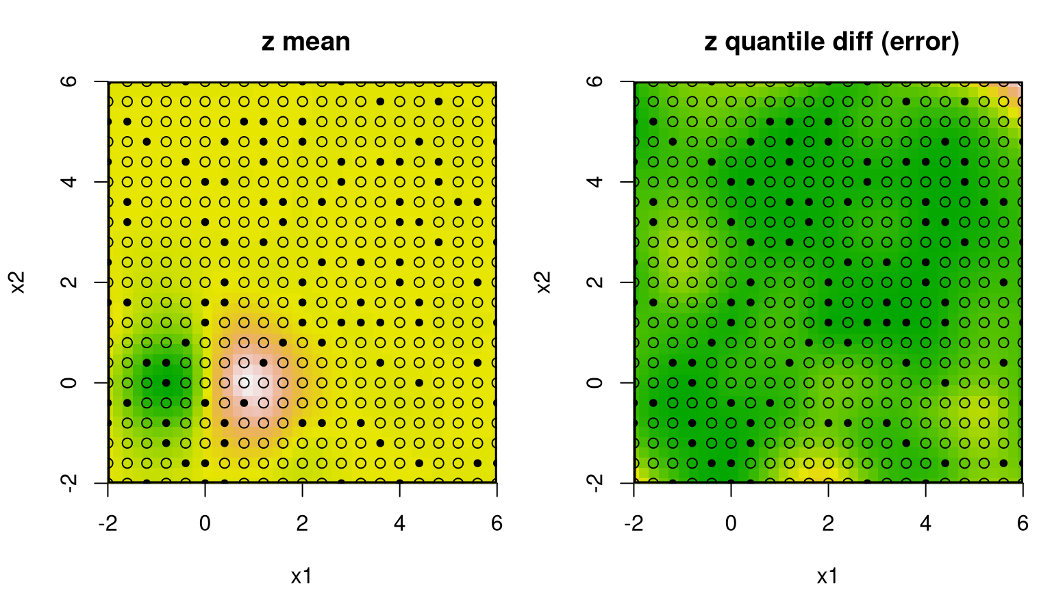
FIGURE 9.13: Bayesian GP fit to the 2d exponential data (§5.1.2) via mean (left) and uncertainty (right; difference between 95% and 5% quantiles).
Occasionally the predictive mean surface (left panel) is exceptionally poor, depending on the random design and response generated by exp2d.data. The predictive variance (right) almost always disappoints. That’s because the GP is stationary which implies, among other things, uniform uncertainty in distance. Consequently, the uncertainty surface is unable to reveal what is intuitively obvious from the pictures: that the interesting quadrant is harder to predict than the other flat ones. The uncertainty surface is sausage-shaped: higher where training data is scarce. To learn otherwise requires building in a degree of nonstationary flexibility, which is what the tree in TGP facilitates. Consider the analogous btgp fit, with modest restarting to avoid the Markov chain becoming stuck in local posterior modes. With GPs at the leaves, rather than constant or linear models, trees are less deep so tree movement is more fluid.
Analogous plots of posterior predictive mean and uncertainty reveal a partition structure that quarantines the interesting region away from the rest, and learns that uncertainty is indeed higher in the lower-left quadrant in spite of denser sampling there. Dashed lines in Figure 9.14 correspond to the MAP treed partition found during posterior sampling.
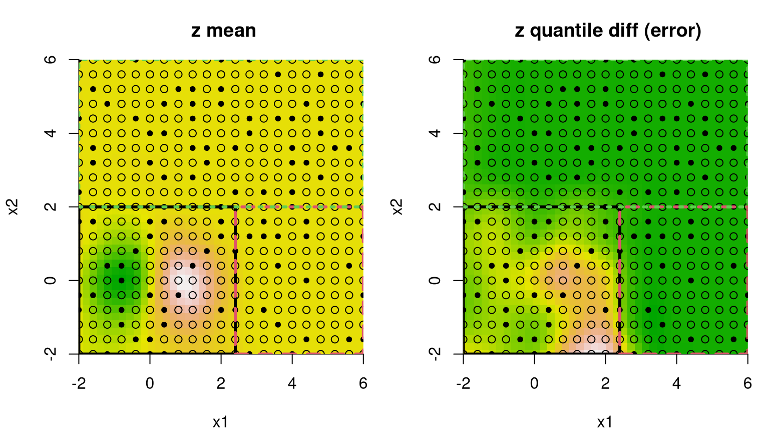
FIGURE 9.14: Bayesian treed GP fit to the 2d exponential data; compare to Figure 9.13.
Recursive axis-aligned partitioning is both a blessing and curse in this example. Notice that one of the flat quadrants is needlessly partitioned away from the other two. But the view in the figure only depicts one, highly probable tree. Posterior sampling averages over many other trees. In fact, a single accepted swap move would result in the diametrically opposed quadrant being isolated instead. This averaging over disparate, highly probable partitions explains why variance is about the same in these two regions. Unfortunately, there’s no support for viewing all of these trees at once, which would anyways be a mess.
Increased uncertainty for the lower-left quadrant in the right panel of Figure 9.14 is primarily due to the shorter lengthscale and higher nugget estimated for data in that region, as supported by many of the trees sampled from the posterior, particularly the MAP. The diagram in Figure 9.15 provides another visual of the MAP tree, relaying a count of the number of observations in each leaf and estimated marginal variance therein.
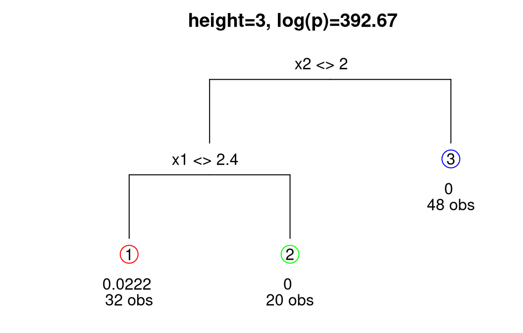
FIGURE 9.15: MAP tree under Bayesian treed GP. Leaf information includes an estimate of local scale (equivalent to \(\hat{\tau}^2\)) and number of observations.
Again, the tree indicates that only the lower-left quadrant has substantial uncertainty. Having a regional notion of model inadequacy is essential to sequential design efforts which utilize variance-based acquisition. Examples are ALM/C, IMSPE, etc., from Chapter 6. All those heuristics are ultimately space-filling unless the model accommodates nonstationary flexibility. A homework exercise in §9.4 targets exploration of these ideas on the motivating NASA rocket booster data (§2.1). In an earlier §6.4 exercise we manually partitioned these data to affect sequential design decisions and direct acquisition towards more challenging-to-model regimes. TGP can take the human out of that loop, automating iteration between flexible learning and adaptive design.
Revisiting LGBB (rocket booster) data
TGP was invented for the rocket booster data. NASA scientists knew they needed to partition modeling, and accompanying design, to separate subsonic and supersonic speeds. They had an idea about how the partition might go, but thought it might be better if the data helped out. Below we shall explore that potential with data collected from a carefully implemented, sequentially designed, computer experiment conducted on NASA’s Columbia supercomputer.
lgbb.as <- read.table("lgbb/lgbb_as.txt", header=TRUE)
lgbb.rest <- read.table("lgbb/lgbb_as_rest.txt", header=TRUE)
Those files contain training input–output pairs obtained with ALC-based sequential design (§6.2.2) selected from a dense candidate grid (Gramacy and Lee 2009). Un-selected elements from that grid form a testing set on which predictions are desired. Here our illustration centers on depicting the final predictive surface, culminating after a sequential design effort on the lift output, one of six responses. The curious reader may wish to repeat this analysis and subsequent visuals with one of the other five output columns. Code below sets up the data we shall use for training and testing.
##     X    XX
##   780 37128
The training set is modestly sized and the testing set is big. Fitting isn’t speedy, so we won’t do any restarts (using default R=1). Even better results can be obtained with larger R and with more MCMC iterations, which is controlled with the BTE argument (“B”urn-in, “T”otal and thinning level to save “E”very sample). Defaults used here target fast execution, not necessarily ideal inferential or predictive performance. CRAN requires all coded examples in documentation files finish in five seconds. This larger example has no hope of achieving that speed, however results with the defaults are acceptable as we shall see.
## elapsed
##   138.5
A fitting time of 138 minutes is quite a wait, but not outrageous. Compared to CSK timings from earlier, these btgpllm calculations are slower even though the training data entertained here is almost an order of magnitude smaller. The reason is that our “effective” covariance matrices from treed partitioning aren’t nearly as sparse. We entertained CSKs at 99% and 99.9% sparsity but our btgpllm MAP tree yields effective sparsity closer to 30%, as we illustrate below. Also, keep in mind that tgp bundles fitting and prediction, and our predictive set is huge. CSK examples entertained just five-hundred predictive locations.
Figure 9.16 provides a 2d slice of the posterior predictive surface where the third input, side-slip angle (beta), is fixed to zero. The plot.tgp method provides several hooks that assist in 2d visualization of higher dimensional fitted surfaces through slices and projections. More details can be found in package documentation.
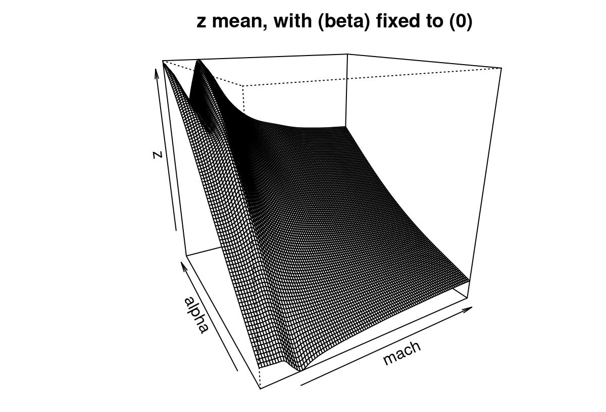
FIGURE 9.16: Slice of the Bayesian TGP with LLM predictive surface for the LGBB lift response.
Observe that the predictive mean surface is able to capture the ridge nearby low speeds (mach) and for high angles of attack (alpha), yet at the same time furnish a more slowly varying surface at higher speeds. That would not be possible under a stationary GP: one of the two regimes (or both) must compromise, and the result would be an inferior fit.
The MAP tree, visualized in Figure 9.17, indicates a two-element partition.
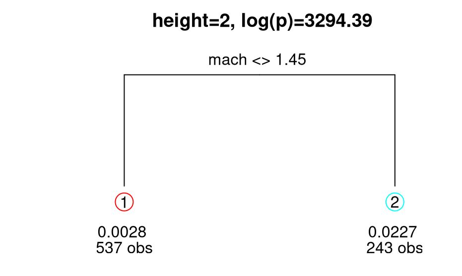
FIGURE 9.17: MAP tree for the lift response.
The number of data points in each leaf implies an effective (global) covariance matrix that’s about 30% sparse, with the precise number depending on the random seed used to generate this Rmarkdown build. Code for a more precise calculation – for a more interesting case with more leaves – is provided momentarily. Note this applies only for the MAP tree; the other thousands of trees visited by the Markov chain would likely be similar but seldom identical.
By default, bt* fitting functions begin with a null tree/single leaf containing all of the data, implying a 100% dense \(780 \times 780\) covariance matrix. So the first several hundred iterations of MCMC, before the first grow move is accepted, may be particularly slow. Even after successfully accepting a grow, subsequent prunes entertain a full \(780 \times 780\), covariance matrix when evaluating MH acceptance ratios. Thus the method is still in \(\mathcal{O}(N^3)\), pointing to very little improvement on computation, at least in terms of computational order. A more favorable assessment would be that we get enhanced fidelity at no extra cost compared to a (dense covariance) stationary GP. More aggressive use of the tree is required when speed is a priority. But let’s finish this example first.
A slightly tweaked plot.tgp call can provide the predictive variance surface. See Figure 9.18. As in our visuals for the 2d exponential data (e.g., Figure 9.14), training inputs (dots) and testing locations (open circles) are shown automatically. A dense testing grid causes lots of open circles to be drawn, which unfortunately darkens the predictive surface. Adding pXX=FALSE makes for a prettier picture, but leaves the testing grid to the imagination. (Here, that grid is pretty easy to imagine in the negative space.) The main title says “z ALM stats”, which should be interpreted as “variance of the response(s)”. Recall that ALM sequential design from §6.2.1 involves a maximizing variance heuristic.
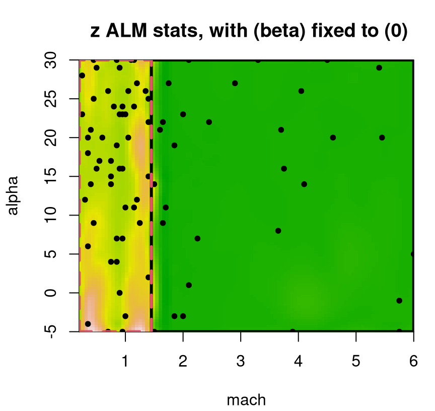
FIGURE 9.18: Predictive uncertainty surface for a slice of the lift response with MAP partition and training data (in slice) overlayed.
Several notable observations can be drawn from this surface. First, the partition doesn’t split the input space equally in a geographic sense. However it does partition the 780 inputs somewhat more equally. This is because the design is non-uniform, emphasizing low-speed inputs. Sequential design was based on ALC, not ALM, but since both focus on variance they would recommend similar acquisitions. Observe that predictive uncertainty is much higher in the low-speed regime, so future acquisitions would likely demand even heavier sampling in that region. In the next iteration of an ALC/M scheme, one might select a new run from the lower-left (low mach, low alpha) region to add into the training data. Finally, notice how high uncertainty bleeds across the MAP partition boundary – a relic of uncertainty in the posterior for \(\mathcal{T}\).
The tgp package provides a number of “knobs” to help speed things up at the expense of faithful modeling. One way is through the prior. For example, \(p_{\mathrm{split}}\) arguments \(\alpha\) (bigger) and \(\beta\) (smaller) can encourage deeper trees and consequently smaller matrices and faster execution.
Another way is through MCMC initialization. Providing linburn=TRUE will burn-in treed GP MCMC with a treed linear model, and then switch-on GPs at the leaves before collecting samples. That facilitates two economies. For starters it shortcuts an expensive full GP burn-in while waiting for accepted grow moves to organically partition up the input space into smaller GPs. More importantly, it causes the tree to over-grow, ensuring smaller partitions, initializing the chain in a local mode of tree space that’s hard to escape out of even after GPs are turned on. Once that happens some pruning is typical, but almost never entirely back to where the chain should be under the target distribution. You might say that linburn=TRUE takes advantage of poor tree mixing, originally observed by CGM, to favor speed.
Consider a btgpllm call identical to the one we did above, except with linburn=TRUE.
As you can see in Figure 9.19, our new visual of the beta=0 slice is not much different than Figure 9.16’s ideal fit. Much of the space is plausibly piecewise linear anyway, but it helps to smooth out rough edges with the GP.
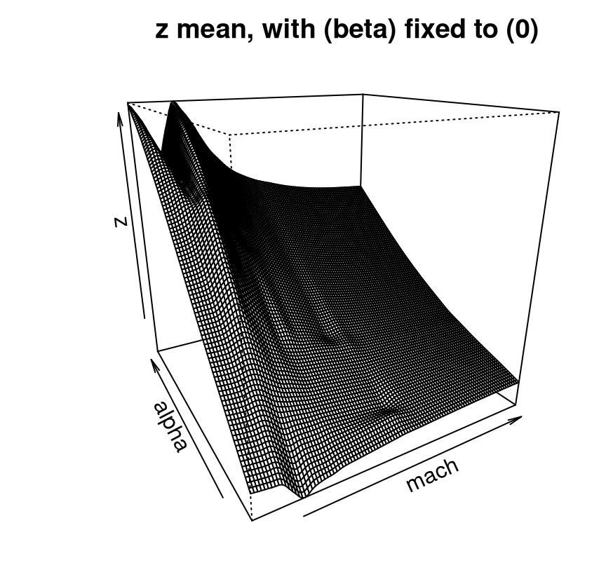
FIGURE 9.19: Approximate LGBB lift posterior mean slice under linear model burn-in; compare to Figure 9.16.
It’s difficult to speculate on the exact nature of the aesthetic difference between this new linburn=TRUE surface and the earlier ideal one. Sometimes the thriftier surface over-smooths. Sometimes it under-smooths revealing kinks or wrinkles. Sometimes it looks pretty much the same. What is consistent, however, is that nothing looks entirely out of place while execution time is about 29 times faster than otherwise, taking about 5 minutes in this build.
##    full.elapsed linburn.elapsed
##          8309.8           287.5
To explain the speedup, code below calculates the effective degree sparsity realized by the MAP tree.
map.height <-fit2$post$height[which.max(fit2$posts$lpost)]
leafs.n <- fit2$trees[[map.height]]$n
1 - sum(leafs.n^2)/(sum(leafs.n)^2)
## [1] 0.9314Approximately 93% sparse – much closer to the 99% of CSK. Maybe its predictive surface isn’t as smooth as it could be, or as would be ideal, say for a final visualization in a published article. For most other purposes, however, linburn fits possess all of the requisite ingredients.
One such purpose is sequential design, where turning around acquisitions quickly can be essential to applicability. We already talked about ALM: an estimate of predictive variance at XX locations comes for free. Usually, although not in all Rmarkdown builds, the ALM/variance surface plotted in Figure 9.20 demands future acquisitions in the interesting part of the space, for low speeds and high angles of attack. Even when that’s not the case, the maximizing location is usually sensible. An important thing to keep in mind about sequential design, especially when individual decisions seem erratic, is that the long run of many acquisitions is what really counts.
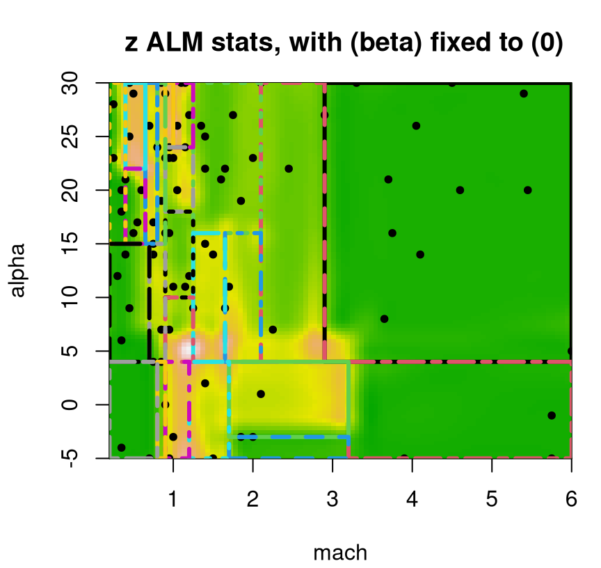
FIGURE 9.20: Approximate LGBB lift posterior mean slice under linear model burn-in; compare to Figure 9.16.
Having to specify XX locations in advance rules out continuous optimization of acquisition criteria, say with optim. Gramacy and Lee (2009) describe a sequential treed maximum entropy (ME) candidate-based scheme for coping with this drawback. The essence is to seek space-filling candidates separately in each region of the MAP partition. ALC (§6.2.2) is available via Ds2x=TRUE, signaling calculations of integrated change in variance \(\Delta \sigma^2(x)\) for all \(x \in\) XX. Testing XX locations are also used as reference sites in a sum approximating the ALC integral (6.7). This makes the computational expense quadratic in nrow(XX), which can be a tall order for testing sets sized in the tens of thousands \((780^3 \ll 37128^2)\). Treed ME XX thus prove valuable as reference locations as well. Finally, additional computational savings may be realized by undoing some of tgp’s defaults, such as automatic predictive sampling at training X locations. Those aren’t really necessary for acquisition and can be skipped by providing pred.n=FALSE.
Often simple leaf models, e.g., constant or linear, lead to great sequential designs. Variance estimates can be quite good, on relative terms, even if predictive means are unfaithful to dynamics exhibited by the response surface. Consequently ALM/C heuristics work quite well. You don’t need smooth prediction to find out where model uncertainty (predictive variance) is high. Consider the treed linear model …
… and resulting ALM surface provided in Figure 9.21. Treed partitioning can be quite heavy, so option pparts=FALSE suppresses those colorful rectangles to provide a clearer view of spatial variance.
plot(fit3, slice=list(x=3,z=0), gridlen=c(100,100), layout="as", as="alm",
  span=0.01, pparts=FALSE, pXX=FALSE)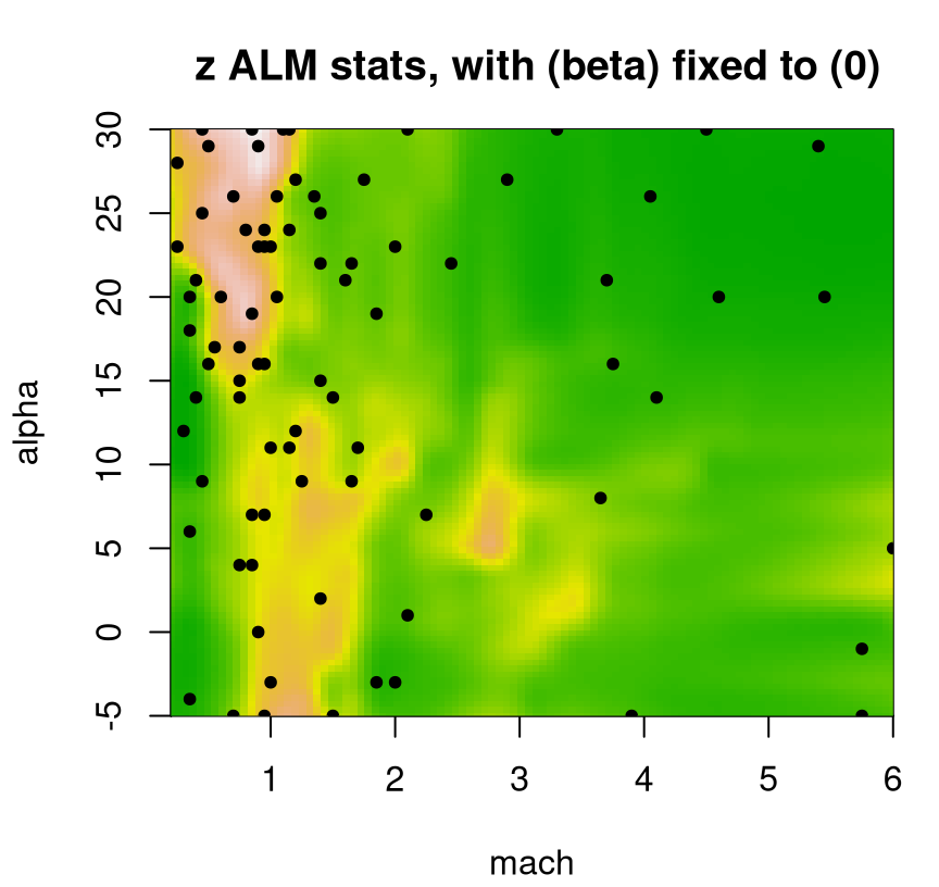
FIGURE 9.21: Even more approximate predictive uncertainty surface under a Bayesian treed LM for a slice of the lift response; compare to Figures 9.18 and 9.20.
That surface indicates a sufficiently localized sense of uncertainty despite having, what would most certainly be, a highly discontinuous (and thus potentially quite inaccurate) predictive mean analog. Despite a factor of R=10 more MCMC sampling, that fit takes a fraction of the time: 1 minute(s), which is 100 times faster than a full TGP.
##    full.elapsed linburn.elapsed    btlm.elapsed
##         8309.82          287.49           82.83
Sometimes treed LMs provide even better acquisitions than treed GPs do. In my experience, this only happens in the latter stages of sequential design. Early on, GP smoothness – at least in part – is key to sensible acquisition. Linear models only have high variance at the edges, i.e., at partition boundaries, which can cause self-reinforcing acquisitions and trigger a vicious cycle. Boundary-targeting sequential design puts a heavy burden on tree mixing in the MCMC, which CGM remind is problematic for linear and constant leaves. If speed is a concern, my preference is for a treed GP with linburn=TRUE shortcuts over wholesale treed linear or constant models. Treed LM burn-in offers a nice compromise: fast predictions and design estimates; smoothed out rough edges, reducing spurious variances due to “over-quilted” input spaces arising from deep trees compensating for crude linear fits at the leaves.
9.2.3 Regression tree extensions, off-shoots and fix-ups
The tgp package also supports expected improvement (EI) for Bayesian optimization (BO; §7.2). Providing improv=TRUE to any b* function causes samples to be gathered from the posterior mean of improvements, converted from raw improvement \(I(x)\) using \(Y(x)\) sampled from the posterior predictive distribution. So you get a fully Bayesian EI, averaged over tree and leaf model uncertainty, for a truly Bayesian BO. (Before the “B” in BO meant marginalizing over a GP latent field; see §5.3.2. Here it means averaging over all uncertainties through posterior integration over the full set of unknown parameters, including trees.) A downside is that candidates, as with other Bayesian TGP sampling of active learning heuristics (ALC/M), must be specified in advance of sampling, thwarting acquisition by local optimization. The upside is that such sampling naturally extends to powered up improvements, encouraging exploration, and ranking by improvement for batch sequential optimization (Taddy et al. 2009).
For more details on tgp, tutorials and examples, see
- Gramacy (2007): a beginner’s primer, including instruction on custom compilation for fast linear algebra and threaded prediction for large
XX, e.g., for LGBB; also seevignette("tgp")in the package; - Gramacy and Taddy (2010): advanced topics like EI, categorical inputs (Broderick and Gramacy 2011), sensitivity analysis, and importance tempering (Gramacy, Samworth, and King 2010) to improve MCMC mixing; also see
vignette("tgp2")in the package.
Several authors have further extended TGP capability. Konomi et al. (2017) demonstrate a nonstationary calibration framework (§8.1) based on TGP. MATLAB® code is provided as supplementary material supporting their paper. Classification with TGP, utilizing a logit linked multinomial response model paired with latent (treed) GP random field, has been explored (Broderick and Gramacy 2011). However synergy between tree and GP is weaker here than in the regression context. Notions of smoothness are artificial when classification labels are involved. A GP latent field can mimic tree-like partitioning features without the help of the tree. Yet the authors were able to engineer some examples where their hybrid was successful.
Another popular approach to tree regression is to combine many simple trees additively. This idea was first introduced in ML as boosting decision stumps. Perhaps the most popular such implementation is gradient tree boosting. See the gbm package (Greenwell, Boehmke, and Cunningham 2019), originally from Ridgeway (2007), and xgboost (Chen et al. 2019) on CRAN. More recently, Bayesian additive regression trees (BART) from CGM (HA Chipman, George, and McCulloch 2010) has gained traction as a sampling-based alternative offering better UQ which can be key in surrogate modeling applications such as BO. Although BART has a built-in additive error model, tweaks can be applied in order to mimic sausage-shaped error-bars when modeling deterministic computer simulations (HA Chipman, Ranjan, and Wang 2012). Several R packages support BART, including BayesTree (Hugh Chipman and McCulloch 2016) and BART (McCulloch et al. 2019), with the latter accommodating a multitude of response types. The space of BART research is quite active and I’d expect many new developments in future. Perhaps the only downside to BART is that predictive surfaces are pathologically non-smooth. Its additive structure does however lend great flexibility and reactiveness to the mean surface which is a substantial asset.
Dynamic trees [DTs; Taddy, Gramacy, and Polson (2011)] were developed specifically to target sequential applications, such as arise in computer simulation, active learning, and BO, with additional support for input importance and sensitivity analysis (§8.2) applications (Gramacy, Taddy, and Wild 2013). An implementation is provided by dynaTree (Gramacy, Taddy, and Anagnostopoulos 2017) on CRAN. DT development revisits the tree prior as a process evolving sequentially in time, and extends that prior to posterior updates as new data arrive. A new data point \((x_{t+1}, y_{t+1})\) may support tree growth or pruning, or neither in favor of the status quo. Inference for DT processes is facilitated by the sequential Monte Carlo method of particle learning (Carvalho et al. 2010). Dynamic trees have been applied on a wide variety of computer surrogate modeling tasks such as computer code semantic translation and autotuning (Balaprakash et al. 2013; Balaprakash, Gramacy, and Wild 2013), stochastic control for epidemic management, financial options pricing, and autonomous vehicle tracking (Gramacy and Ludkovski 2015). Streaming applications, which deploy data point retirement in order to work in fixed memory and forgetting factors in the face of concept drift (a target response surface that’s evolving in time), are described by Anagnostopoulos and Gramacy (2013).
For applications which are not inherently sequential in nature, DTs can be applied to random data orderings. Randomization over the “arrival-time” of data has a simultaneous bootstrap and likelihood annealing effect. The results are, at least in some cases, astounding. Consider the following multiple DTs (dynaTrees) fit to mcycle data (§9.2.1), separately under constant and linear leaves.
XX <- seq(0,max(mcycle[,1]), length=1000)
out.dtc <- dynaTrees(X=mcycle[,1], y=mcycle[,2], XX=XX, verb=0, pverb=0)
out.dtl <- dynaTrees(X=mcycle[,1], y=mcycle[,2], XX=XX, model="linear",
  verb=0, pverb=0)
Unfortunately the structure of the output objects doesn’t align with tgp so we can’t use the plotting macro from earlier. Similar code, evaluated below, aggregates means and quantiles extracted from 1000 random re-passes through the data.
plot(out.dtc$XX[,1], rowMeans(out.dtc$mean), type="l", ylim=c(-160, 110),
  ylab="accel", xlab="time")
points(mcycle)
lines(out.dtc$XX[,1], rowMeans(out.dtc$q1), lty=2)
lines(out.dtc$XX[,1], rowMeans(out.dtc$q2), col=1, lty=2)
lines(out.dtl$XX[,1], rowMeans(out.dtl$mean), col=2)
lines(out.dtl$XX[,1], rowMeans(out.dtl$q1), col=2, lty=2)
lines(out.dtl$XX[,1], rowMeans(out.dtl$q2), col=2, lty=2)
legend("topleft", legend=c("DT constant", "DT linear"), bty="n",
  lty=1, col=1:2)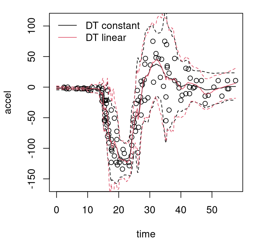
FIGURE 9.22: Dynamic trees posterior predictive surfaces on the motorcycle accident data.
The first time I saw these plots I was blown away. Aesthetically, constant leaves seem to offer better compromise between dynamic reactivity and smoothing. But how can piecewise constant models look so smooth, on average, but still mimic abrupt features in the data? Bootstrap aggregation, or bagging, which manifests as random data orderings in DT, is a powerful tool. Bagging is the workhorse behind random forest (RF) models, supported by several packages including randomForest (Breiman et al. 2018) on CRAN. Indeed, RFs make similarly strong surrogates, however extracting full predictive uncertainty can be challenging. A review paper by H. Chipman et al. (2013) provides more in-depth qualitative and quantitative comparison between Bayesian (and classical) tree-based regression methods. In fairness, not all examples (whether via dynaTree, bcart, btlm or BayesTree) look as good as the mcycle ones presented here. GPs are hard to beat in bakeoffs spanning diverse data-generating mechanisms, input dimensions and sizes (so long as the calculations remain computationally tractable).
Finally, tessellation-based partition modeling has been revisited from several angles in recent literature. Rushdi et al. (2017) provide new data structures and new computational approaches to shortcut expensive search subroutines required for prediction under Voronoi piecewise surrogates. C. Park and Apley (2018) consider patching together piecewise fits to furnish a degree of smoothness across partition boundaries. Rullière et al. (2018) propose a nested approach to divide-and-conquer modeling. Those are just a few, non-representative examples; I doubt we’ve heard the last word on partition-based regression and surrogate modeling. Divide-and-conquer remains an attractive device for marrying computational thrift with modeling fidelity.
9.3 Local approximate GPs
A local approximate Gaussian process (LAGP), which I’ve been so excited to tell you about for hundreds of pages, has aspects in common with partition based schemes, in the sense that it creates sparsity in the covariance structure in a geographically local way. In fact, LAGP is a partitioning scheme in a limiting sense, although delving too deeply into that connection is counterproductive because the approach is quite different from partitioning in spirit. The core LAGP innovation is reminiscent of what Cressie (1992, 131–34) called “ad hoc local kriging neighborhoods”. Perhaps in 1992 the basic idea, which at face value isn’t mind blowing but might have gotten less credit than it deserves, was simply a little ahead of its time. I think that the geostatistical community of that era may not have anticipated the scale of modern data, a ubiquity of applications to computer simulation and ML (with inputs other than longitude and latitude), and the architecture of contemporary supercomputers. Multi-core/cluster parallelization begs for divide-and-conquer.
All in all, LAGP’s building blocks and their synthesis are more modern, both technologically and culturally, than could have been anticipated thirty-odd years ago. Technology wise, it draws on recent findings for approximate likelihoods in spatial data (e.g., Stein, Chi, and Welty 2004), and active learning techniques for sequential design (e.g., Cohn 1994). But the big divergence, particularly from geostatistics, is cultural. Interest in LAGP lies squarely in prediction, which is the primary goal in computer experiments and ML applications.
Although designed for large-scale statistical surrogate modeling, the LAGP mindset is distinctly ML. The methodology is an example of transductive learning (Vapnik 2013), with training tailored to predictive goals. This is as opposed to the more familiar inductive sort, where model fitting and prediction transpire in serial, usually in two distinct stages. A transductive learner utilizes training data differently depending on where prediction is required and to what end predictions might be used. Consequently the enterprise is more about reaction, decision and adaptation than it is about inference.
9.3.1 Local subdesign
For the next little bit, focus on prediction at a single testing location \(x\). Coordinates encoded by \(x\) are arbitrary; it’s only important that it be a single location in the input space \(\mathcal{X}\). Let’s think about the properties of a GP surrogate at \(x\). Training data far from \(x\) have vanishingly small influence on GP predictions, especially when correlation is measured as an inverse of exponentiated Euclidean distances. This is what motivates a CSK approach to inducing sparsity (§9.1), but the difference here is that we’re thinking about a particular \(x\), not the entire spatial field.
The crux of LAGP is a search for the most useful training data points – a subdesign relative to \(x\) – for predicting at \(x\), without considering/handling large matrices. One option is a nearest neighbor (NN) subset. Specifically, fill \(X_n(x) \subset X_N\) with \(\mbox{local-}n \ll \mbox{full-}N\) closest locations to \(x\). Notice that I’ve tweaked notation a bit to have big \(N\) represent the size of a potentially enormous training set, unwieldy for conventional GPs, and now little \(n\) denotes a much smaller, more manageable size. Derive GP predictive equations under \(Y(x) \mid D_n(x)\) where \(D_n(x) = (X_n, Y_n)\), pretending that no other data exist. The best reference for this idea is Emery (2009). This prediction rule is as simple to implement as it is to describe, and it’s very fast on relative terms when \(n \ll N\). Costs are in \(\mathcal{O}(n^3)\) and \(\mathcal{O}(n^2 + N)\) for decomposition(s) and storage, respectively; and NNs can be found in \(\mathcal{O}(n \log N)\) time with k-d trees after an up-front \(\mathcal{O}(N \log N)\) build cost. In practice, one can choose local-\(n\) as large as computational constraints allow, although there may be reasons to prefer smaller \(n\) on reactivity grounds. Predictors may potentially be more accurate at \(x\) if they’re not burdened by information from training data far from \(x\).
This is different, and much simpler than, what other authors have recently dubbed nearest neighbor GP regression [NNGP; Datta et al. (2016)], which is a potential source of confusion. NNGP is clever, but targets global rather than local inference and prediction. The way in which neighbors are used is not akin to canonical NN, i.e., nonparametric regression and classification where each testing prediction conditions only on a small set of very closest training points. Neighborhood sets in NNGP, rather, anchor an approximate Cholesky decomposition leading to a joint distribution similar to what could be obtained at greater computational expense under a full conditioning set. This so-called Vecchia approximation (Vecchia 1988; Stroud, Stein, and Lysen 2017) induces sparsity in the inverse covariance structure. After this fashion, NNGP might be more aptly named “Bayesian Vecchia”. Also see Katzfuss and Guinness (2018) for a more general treatment of conditioning sets toward that end. Both groups of authors provide implementations on CRAN; see spBayes (A. Finley and Banerjee 2019) and GpGp (Guinness and Katzfuss 2019), respectively. Empirical performance with these packages, tackling large geospatial data and furnishing accurate predictions and estimates of uncertainty, is impressive. As far as I know, they’re untested in (higher dimensional) computer surrogate modeling and ML contexts.
Ok, apologies for the short digression. The essence of NN-based local GP approximation, using as training data that \(D_n(x)\) which is closest to predictive location \(x\), is embodied by the cartoon in Figure 9.23. Gridded black dots represent a massive training design \(X_N\). There are mere thousands of such dots in the grid, but imagine hundreds of thousands or millions. Five solid, colored dots in the figure represent potential \(x\) sites. Open circles of the same color indicate NN subdesigns \(X_n(x) \subset X_N\) corresponding to those predictive locations.
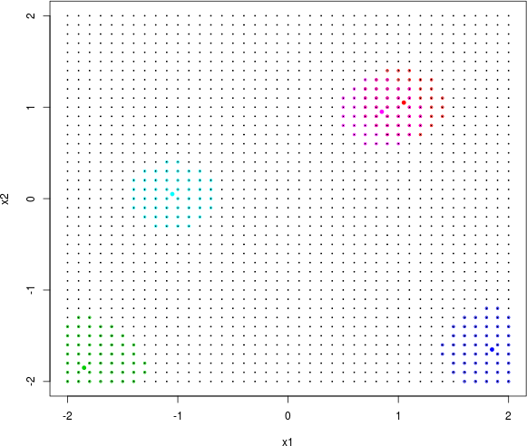
FIGURE 9.23: Local neighborhoods (colored open circles) based on NN subdesign for predictive locations (colored filled dots) as selected from a large design (small black dots).
Notice how topology of the global design \(X_N\) impacts the shape of local designs \(X_n(x)\). When two predictive locations are nearby, as illustrated in pink and red, training data sites may be shared by subdesigns. There are no hard boundaries whereby adjacent, arbitrarily close predictive locations might be trained on totally disjoint data subsets. It’s even possible to have two very close predictive locations \(x \ne x'\) with the same subdesign \(X_n(x) = X_n(x')\) when they share the same NN sets.
What can be said about this NN-based GP approximation? Is it sensible? Under fixed hyperparameterization and some regularity conditions that would be a distraction to review, one can show that as \(n \rightarrow N\) predictions \(Y(x) \mid D_n \rightarrow Y(x) \mid D_N\). In other words, larger local design size means better approximation. Being endowed with the label “approximate” requires some notion of accuracy relative to an exact alternative. It can also be shown, again under some regularity conditions, that \(V(x) \mid D_n \gg V(x) \mid D_N\), reflecting uncertainties inflated by the smaller design, where \(\sigma^2(x) = \hat{\tau}^2 V(x)\).
Is it good? Empirically, yes, but it’s not optimal given computational limits, \(n\) (Vecchia 1988; Stein, Chi, and Welty 2004). Of all size-\(n\) subsets of \(N\) training data sites, those residing closest to \(x\) in terms of Euclidean distance are not optimal for predicting at \(x\). Clearly it’s good to have some, perhaps many, nearby training sites. However, some farther out sites – not included because they’re not part of the NN set – may be useful as anchors, providing long-range spatial dependence information. That information is potentially of greater value because it’s less correlated/more independent than that which is provided by closer-in points. (If we already have a bunch of nearby points, the marginal value of another one has diminishing returns. It could be better to have independent information farther out.) That being said, finding the optimal \(n\) of \(N\), of which there are \({N \choose n}\) alternatives, could be a combinatorially huge undertaking.
So that begs the question: can we do better than NN (in terms of prediction accuracy) without much extra effort (in terms of computational cost)? More precisely, \(n\)-NN GP prediction requires computation in \(\mathcal{O}(n^3)\). So can we find a dataset \(D_n(x)\), using time in \(\mathcal{O}(n^3)\) combining search, hyperparameter inference, and prediction, where accuracy at \(x\) based on that set is no worse than under \(D_n^{\mathrm{(NN)}}(x)\), the NN special case? Of course by “no worse” I really mean “hopefully much better”, but choose to manage expectations by phrasing things conservatively.
The answer to that question is a qualified “Yes!”, with a greedy/forward stepwise scheme. For a particular predictive location \(x\), solve a sequence of easy decision problems.
For \(j=n_0, \dots,n\):
- given \(D_j(x)\), choose \(x_{j+1}\) according to some criterion;
- augment the design \(D_{j+1}(x) = D_j(x) \cup (x_{j+1}, y(x_{j+1}))\) and update the GP approximation.
Optimizing the criterion (1), and updating the GP (2), must not exceed \(\mathcal{O}(j^2)\) so the total scheme remains in \(\mathcal{O}(n^3)\). Initialize with a small \(D_{n_0}(x)\) comprised of NNs.
Gramacy and Apley (2015), G&A below, proposed the following criterion for sequential subdesign. Given \(D_j(x)\) for particular \(x\), search for \(x_{j+1} \in X_N \setminus X_n(x)\) considering its impact on predictive variance \(V_j(x) \equiv V(x) \mid D_j(x)\), while taking into account uncertainty in hyperparameters \(\theta\), by minimizing empirical Bayes mean-squared prediction error:
\[\begin{align} J(x_{j+1}, x) &= \mathbb{E} \{ [Y(x) - \mu_{j+1}(x; \hat{\theta}_{j+1})]^2 \mid D_j(x) \} \notag \\ &\approx V_j(x \mid x_{j+1}; \hat{\theta}_j) + \left(\frac{\partial \mu_j(x; \theta)}{\partial \theta} \Big{|}_{\theta = \hat{\theta}_j}\right)^2 \Big{/}\, \mathcal{G}_{j+1}(\hat{\theta}_j). \tag{9.2} \end{align}\]
The approximation stems from Gaussian instead of Student-\(t\) predictive equations, and plugging in estimated kernel hyperparameters \(\hat{\theta}_j\) instead of \(\hat{\theta}_{j+1}\). Student-\(t\) equations arise upon estimating, or integrating out, the covariance scale \(\tau^2\). This detail is glossed over in our Chapter 5 introduction; since predictive equations presented therein were Gaussian, these were technically an approximation as well. As \(N\), or in this context \(n\), gets larger (\(\gg 30\), say), the approximation error is small. Plugging in \(\hat{\theta}_j\) for \(\hat{\theta}_{j+1}\) avoids entertaining how estimated lengthscales might change as new \(y_{j+1}\) are incorporated, depending on the selected \(x_{j+1}\) location. In practice \(\theta\) is fixed throughout sequential design iterations; more implementation details will be covered later.
Let’s break down elements of the MSPE criterion \(J(x_{j+1}, x)\). Apparently it combines variance and rate of change of the mean at \(x\). G&A’s presentation, and indeed the original laGP package implementation (Gramacy and Sun 2018), emphasized isotropic lengthscale parameters \(\theta\). Our summary here follows that simplified setup. For extensions to vectorized \(\theta\) for separable, coordinate-wise, lengthscales see the appendix to the original paper. A subsequently updated version of laGP supports separable lengthscales, as detailed by our empirical work below.
The first part of \(J\), namely \(V_j(x \mid x_{j+1}; \theta)\), is our old friend: an estimate of the new variance that will result after adding \(x_{j+1}\) into \(D_j\), treating \(\theta\) as known.
\[ \begin{aligned} V_j(x \mid x_{j+1}; \theta) &= \frac{\psi_j}{j-2} v_{j+1}(x; \theta), \\ \mbox{where } \;\;\; v_{j+1}(x; \theta) &= \left[ K_{j+1}(x, x) - k_{j+1}^\top(x) K_{j+1}^{-1} k_{j+1}(x) \right] \;\;\; \mbox{and } \;\;\; \psi_j = j \hat{\tau}^2_j. \end{aligned} \]
Integrating \(V_j(x|x_{j+1}; \theta)\) over \(x\) yields the ALC acquisition criterion for approximate global \(A\)-optimal design (Seo et al. 2000; Cohn 1994). §6.3 showed how \(v_{j+1}\) can be updated from \(v_j\), and other quantities available at iteration \(j\), in \(\mathcal{O}(j^2)\) time.
Next, \(\frac{\partial \mu_j(x; \theta)}{\partial \theta}\) is the partial derivative of the predictive mean at \(x\), given \(D_j\), with respect to lengthscale:
\[ \frac{\partial \mu_j(x;\theta)}{\partial \theta} = K_j^{-1}[\dot{k}_j(x) - \dot{K}_j K_j^{-1} k_j(x)]^\top Y_j, \]
where \(\dot{k}_j(x)\) is a length-\(j\) column vector of derivatives of kernel correlations \(K(x, x_k)\), for \(k=1,\dots,j\), taken with respect to \(\theta\). So it’s the rate of change of predictive mean with respect to changes in lengthscale(s). These can be updated in \(\mathcal{O}(j^2)\) too; see G&A for more details.
Finally, \(\mathcal{G}_{j+1}(\theta)\) is also an old friend (§6.2.3): the Fisher information (FI) from \(D_j\), including an expected component from future \(Y_{j+1}\) at \(x_{j+1}\):
\[ \begin{aligned} &\mathcal{G}_{j+1}(\theta) = F_j(\theta) + \mathbb{E} \left\{- \frac{\partial^2 \ell_j(y_{j+1}; \theta)}{\partial \theta^2} \,\Big{|}\, Y_j; \theta \right\} \\ &\approx F_j(\theta) \!+\! \frac{1}{2 V_j(x_{j+1};\theta)^2} \!\times\! \left( \frac{\partial V_j(x_{j+1}; \theta)}{\partial \theta} \right)^2 \!\!+\! \frac{1}{V_j(x_{j+1}; \theta)} \left( \frac{\partial \mu_j(x_{j+1}; \theta)}{\partial \theta} \right)^2\!, \end{aligned} \]
where \(F_j(\theta) = - \ell''(Y_j; \theta)\), and with \(\dot{\mathcal{K}}_j = \dot{K}_j K_j^{-1}\) and \(\tilde{k}_j(x) = K_j^{-1} k_j(x)\),
\[ \begin{aligned} \frac{\partial V_j(x; \theta)}{\partial \theta} & = \frac{Y_j^\top K_j^{-1}\dot{\mathcal{K}}_j Y_j }{j-2} \left(K(x, x) -k_j^\top(x) \tilde{k}_j(x)\right) \\ &\;\;\; - \psi_j\left[ \dot{k}_j(x) \tilde{k}_j(x) + \tilde{k}_j(x)^\top (\dot{k}_j(x)-\dot{\mathcal{K}}_j k_j(x)) \right]. \end{aligned} \]
G&A similarly detail how the derivative of \(V_j\) may be updated in \(\mathcal{O}(j^2)\) time which is nearly identical to our development for \(v_j\) provided in §6.3.
Observe how inverse FI, which for vectorized \(\theta\) would be a matrix inverse and applied in full quadratic form as \((\partial \mu_j)^\top \mathcal{G}_{j+1}^{-1} (\partial \mu_j)\), serves as a weight in a trade-off between variance reduction and sensitivity of predictive mean to hyperparameters \(\theta\). Referring back to our global FI-based sequential design illustration from §6.2.3, FI generally increases as more samples are added. Therefore the weight applied to the second term in the MSPE criterion \(J\) in Eq. (9.2) diminishes as \(j\) increases, effectively up-weighting reduction in variance.
Although MSPE nests an ALC-like criteria (§6.2.2), importantly we don’t need to integrate (or in practice sum) over reference locations. The single testing location \(x\) is our (only) reference location. Reducing future variance is a sensible criterion in its own right, and considering that the FI-based weight acts most strongly for low \(j\), one may wonder whether the extra complication of calculating first and second derivatives is “worth it” for full MSPE? Perhaps ALC on its own – basing sequential subdesign decisions on \(V_j(x \mid x_{j+1}; \theta)\) only – is sufficient to beat the simple NN set. Let’s see how these two alternatives, referred to as MSPE and ALC below, compare qualitatively and empirically in a simple example.
9.3.2 Illustrating LAGP: ALC v. MSPE
Consider a design of size \(N\approx 40,000\) on a 2d grid in \([-2,2]^2\).
## [1] 40401Technically, greedy subdesign search (using ALC or MSPE) doesn’t require a response. Conditional on hyperparameters \(\theta\), calculations involve \(X_N\) and \(x\) only. Still, being engineered to furnish predictions, laGP wants responses \(Y_N\) too, i.e., the full \(D_N\). We’ll be looking at those predictions shortly anyways, so this is as good a time as any to introduce a challenging test problem.
The function below was chosen by G&A because it’s sufficiently complicated to warrant a large training set despite being in relatively small input dimension. Some have taken to calling this “Herbie’s tooth”; it was dreamed up as a challenging Bayesian optimization test problem by Herbie Lee (H. Lee et al. 2011), my PhD advisor, and looks like a molar when plotted in 2d. We used it in §7.3.7 to illustrate an augmented Lagrangian BO method. Although most uses, including the original, are in 2d, the function is sometimes mapped to higher input dimension. Let
\[\begin{equation} g(z) = \exp\left(-(z-1)2\right) + \exp\left(-0.8(z+1)2\right) - 0.05\sin\left(8(z+0.1)\right), \tag{9.3} \end{equation}\]
be defined for scalar inputs \(z\). Then, for inputs \(x\) with \(m\) coordinates \(x_1,\dots,x_m\), the response is \(f(x) = -\prod_{j=1}^m g(x_j)\). Some variations in the literature use \(-f(x)\) instead, depending on whether the application (e.g., optimization) emphasizes minima or maxima. The un-negated version is easier to visualize with perspective plots, as we do shortly.
An implementation is provided below, modified from the §7.3.7 version to handle generic input dimension.
herbtooth <- function(X)
 {
  g <- function(z)
    return(exp(-(z - 1)^2) + exp(-0.8*(z + 1)^2) - 0.05*sin(8*(z + 0.1)))
  return(-apply(apply(X, 2, g), 1, prod))
 }
In spite of that upgrade in generality, we shall apply Herbie’s tooth here, over our large gridded X \(\equiv X_N\), in the easy-to-visualize 2d case. For a four-dimensional application, see Section 4.3 of Sun, Gramacy, Haaland, Lawrence, et al. (2019).
Now consider predictive location \(x\), denoted by Xref in the code below, via local designs constructed greedily based on MSPE and ALC.
library(laGP)
Xref <- matrix(c(-1.725, 1.725), nrow=1)
p.mspe <- laGP(Xref, 6, 50, X, Y, d=0.1, method="mspe")
p.alc <- laGP(Xref, 6, 50, X, Y, d=0.1, method="alc")
As specified by the calls above, both design searches initialize with \(n_0 = 6\) NNs, make greedy selections until \(n = 50\) locations are chosen, and use an isotropic d \(\equiv \theta = 0.1\) hyperparameterized Gaussian kernel. The goal is to interpolate these deterministic evaluations. Although one can specify a zero nugget, a more conservative default setting of g=1e-4 is used to ensure numeric positive-definiteness. When numerics are more favorable, smaller g often leads to better results, as we shall illustrate later in a more ambitious setting. Figure 9.24 shows the resulting selections.
plot(X[p.mspe$Xi,], xlab="x1", ylab="x2", type="n",
  xlim=range(X[p.mspe$Xi,1]), ylim=range(X[p.mspe$Xi,2]))
text(X[p.mspe$Xi,], labels=1:length(p.mspe$Xi), cex=0.7)
text(X[p.alc$Xi,], labels=1:length(p.alc$Xi), cex=0.7, col=2)
points(Xref[1], Xref[2], pch=19, col=3)
legend("right", c("mspe", "alc"), text.col=c(1,2), bty="n")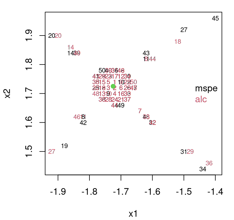
FIGURE 9.24: Comparing LAGP subdesigns under MSPE (9.2) and the ALC special case. The predictive location \(x\) is a filled-green dot. Numbers indicate the order in which each training-data location was greedily selected for the local subdesign.
The green dot is \(x \equiv\) Xref. Each number plotted, whether in red for ALC or black for MSPE, indicates the order in which greedy selections were made. Although the grid of possible candidates \(X_N \setminus X_{n_0}(x)\) is not shown, it’s easy to mentally visualize them filling in the negative space. Notice that there are early selections which are not NNs, and there are late selections which are. The order in which an NN or non-NN is chosen is hard to predict. Non-NN subdesign selections are sometimes called satellite points. Although these satellites are not NNs, they aren’t that far from \(x\) in the entire space, which is \([-2,2]^2\). (Observe that the plotting domain is smaller than the full span of the design \(X_N\).) Finally, any differences between ALC and MSPE are slight at best, at least aesthetically speaking.
Is the result in the figure surprising? Why do the criteria not prefer only the closest possible points, i.e., NNs? An exponentially decaying correlation should substantially devalue locations far from \(x\). Gramacy and Haaland (2016) explain that the form of the correlation has very little to do with it. Consider (scale free) reduction in variance, an expression we’ve seen before (6.9):
\[ v_j(x; \theta) - v_{j+1}(x; \theta) = k_j^\top(x) G_j(x_{j+1}) v_j(x_{j+1}) k_j(x) + \cdots + K(x_{j+1},x)^2 / v_j(x_{j+1}). \]
Although quadratic in inverse distance \(K(x_{j+1},x)^2\), terms are also quadratic in inverse inverse distance, e.g.,
\[ G_j(x') \equiv g_j(x') g_j^\top(x') \quad \mbox{where} \quad g_j(x') = - K_j^{-1} k_j(x')/v_j(x'). \]
So the criteria make a trade-off: minimize scaled distance to \(x\) while maximizing distance (or minimizing inverse distance) to the existing design \(X_j(x)\). Or in other words, the potential value of new design element \((x_{j+1}, y_{j+1})\) depends not just on its proximity to \(x\), but also on how potentially different that information is to where we already have (lots of) it, at \(X_j(x)\).
Both MSPE and ALC provide a mixture of NNs and satellite points. What about the rays, emanating from \(x\), that satellite points seem to arrange themselves around? Those are due to the radial structure of our isotropic kernel. Satellite points would like to be even more radial except that a discrete, gridded \(X_N\) is thwarting that outcome. Gramacy and Haaland show some of the interesting patterns, manifest as ribbons and rings, that materialize in local designs depending on kernel and hyperparameterization.
How about prediction? The two local subdesigns are qualitatively similar. Predictions are, empirically speaking, nearly identical:
p <- rbind(c(p.mspe$mean, p.mspe$s2, p.mspe$df),
  c(p.alc$mean, p.alc$s2, p.alc$df))
colnames(p) <- c("mean", "s2", "df")
rownames(p) <- c("mspe", "alc")
p
## mean s2 df
## mspe -0.3725 2.519e-06 50
## alc -0.3725 2.445e-06 50Despite being built under greedy criteria for fixed lengthscale \(\theta = 0.1\), the predictive equations output by laGP utilize local MLEs based on data subset \(D_n(x)\). That is, after \(n\) selections, \(\hat{\theta}_n(x) \mid D_n(X)\) is calculated before applying the usual GP predictive equations (5.2).
##           d dits
## mspe 0.3589    7
## alc  0.3378    7
These are also nearly identical for the two sequential subdesign criteria. Very few Newton iterations (dits) are required for convergence to \(\hat{\theta}_n(x)\). Finally, both local subdesign searches are fast.
## mspe.elapsed  alc.elapsed
##        0.146        0.042
ALC is about 3\(\times\) faster because it bypasses derivative calculations, motivating that choice as the default in the package. For a point of reference, inverting a \(4000 \times 4000\) matrix takes about five seconds on the same machine, but this can be improved upon with customized linear algebra (Appendix A); an improvement which would be enjoyed by laGP as well. Never mind a \(40,000 \times 40,000\) decomposition – impossible on ordinary workstations.
Calculating an NN subdesign is faster even though the computational order is the same. Constant and lower order (quadratic and linear terms) add substantially to the work required to make greedy ALC selections. Yet calculating MLE \(\hat{\theta}_n(x)\) at the end is what dominates. Table 9.1 summarizes predictive quantities and calculations involved in local lengthscale estimation.
p.nn <- laGP(Xref, 6, 50, X, Y, d=0.1, method="nn")
p <- rbind(p, nn=c(p.nn$mean, p.nn$s2, p.nn$df))
mle <- rbind(mle, nn=p.nn$mle)
ts <- c(ts, nn=p.nn$time)
kable(cbind(p, mle, ts),
caption="Summarizing calculation times in local lengthscale estimation.")| mean | s2 | df | d | dits | ts | |
|---|---|---|---|---|---|---|
| mspe | -0.3725 | 0 | 50 | 0.3589 | 7 | 0.146 |
| alc | -0.3725 | 0 | 50 | 0.3378 | 7 | 0.042 |
| nn | -0.3726 | 0 | 50 | 0.2096 | 6 | 0.004 |
NN is the exception in lengthscale hyperparameter d \(\equiv \hat{\theta}_n(x)\) and speed. NN’s shorter lengthscale can be explained by its more compact subdesign: longer lengthscales require support from (absent) longer pairwise distances. Considering speed differences, it’s worth asking if the extra effort of ALC or MSPE local subdesign is worth it compared to NN. Until we’re able to collect predictions at a suite of testing locations, for many \(x \in \mathcal{X}\), it’s not worth commenting in finer detail on relative accuracies. If you want to take my word for it: for fixed subdesign size \(n\), ALC and MSPE outperform NN. But a more natural comparator is NN based on a bigger \(n' > n\), one requiring a commensurate amount of computational time to compute. That’s a difficult comparison to make, or at least to make fair. See, for example, Section 3.1 of Gramacy (2016) which illustrates that, in at least one view on the borehole data, \(n=50\) ALC-based subdesigns yield predictions that are more accurate than ones based on much larger \(n'=200\) NN local subsets in about the same amount of time.
Complicating things further, there are several mechanisms built into laGP targeting search speedups at the expense of (possibly) less faithful greedy selection. A parameter close adjusts the scope of candidates entertained for local acquisition. Rather than search over all \(X_N \setminus X_j(x)\), one can safely entertain only close \(\equiv N' \ll N\) NNs, say close=1000 (the default), without any effect on the chosen subdesign compared to one obtained under an exhaustive search. Sung, Gramacy, and Haaland (2018) show how an even smaller, but more dynamically determined, set can be entertained by ruling out large swaths of \(X_N \setminus X_j(x)\) as “noncompetitive for selection”. Gramacy, Niemi, and Weiss (2014) demonstrate how greedy selection among tens of thousands of candidates can be off-loaded to a GPU for essentially instantaneous execution; Gramacy and Haaland (2016) illustrate how exhaustive discrete searches over \(X_N \setminus X_j(x)\) can be replaced by simple 1d line searches, along rays emanating from \(x\), whose solutions may be snapped back to the original (un-selected) design locations; finally Sun, Gramacy, Haaland, Lu, et al. (2019) provide a similar – perhaps more exact but also more involved – approach using gradients.
In a nutshell, one can dramatically speed up greedy ALC and MSPE searches with little impact on accuracy, furnishing predictions more accurate than NN in about the same amount of time. All of the methods listed above are built into laGP for ALC (and some also for MSPE). An exercise in §9.4 entertains some of these alternatives alongside defaults. Perhaps the best reason to prefer ALC and MSPE over NN is that G&A show empirically that those methods lead to better numerical conditioning of the resulting \(n \times n\) local covariance matrices. When training data are too close together in the design space, the covariance structure becomes difficult to decompose. Local GP approximation via NN can exacerbate this numerical challenge; satellite points from ALC and MSPE offer some relief. Numerically stable local prediction is a crucial engineering detail to consider in repeated application, say over a dense testing set – which is our next subject.
9.3.3 Global LAGP surrogate
How can this local strategy be extended to predict on a big testing/predictive set \(\mathcal{X}\)? One simple option is to serialize: tack on a for loop over each \(x \in \mathcal{X}\). But why serialize when you can parallelize? Each \(D_n(x)\) is obtained independently of other \(x\)’s, so they may be constructed simultaneously. In laGP’s C implementation, that’s as simple as a parallel for OpenMP pragma.
#ifdef _OPENMP
  #pragma omp parallel for private(i)
#endif
  for(i = 0; i < npred; i++) { ...
It really is that simple. The original implementation in laGP used exactly that pragma. Subsequent versions have upgraded to more elaborate families of pragmas in order to trim overheads inherent in parallel for.
With modern laptops having two hyperthreaded cores (meaning they can run four threads in parallel), and many desktops having eight (16 threads) or more, parallelization in implementation is essential to taking full advantage of contemporary architectures. OpenMP is the simplest way to accomplish shared memory parallelization (SMP) in C and Fortran. Statistically speaking, leveraging SMP means exploiting or introducing statistical independence. Local approximation with LAGP imposes exactly this kind of statistical, and thus algorithmic independence structure already. No further approximation is required in order to predict with laGP in parallel for many \(x\).
To illustrate, consider the following \(\approx 10\)K-element predictive grid in \([-2,2]^2\), spaced to avoid the original \(N\approx 40\)K design.
The aGP function automates “iteration” over elements of \(\mathcal{X} =\) XX, and its omp.threads argument controls the number of OpenMP threads. Here we’ll use 8 threads, even though my desktop is hyperthreaded (can do 16).
## elapsed
##   75.85
Observe that the compute time reflects almost linear scaling by comparison to the time extrapolated for our earlier singleton ALC run.
## elapsed
##   51.46
Figure 9.25 offers a view of the predictive mean surface thus obtained. That surface is negated to ease visibility in this perspective.
persp(xx, xx, -matrix(P.alc$mean, ncol=length(xx)), phi=45, theta=45,
    xlab="x1", ylab="x2", zlab="yhat(x)")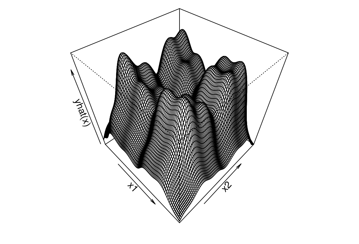
FIGURE 9.25: Global approximation by independent and parallel LAGP predictions on Herbie’s tooth.
Perhaps you can see why this surface is called “Herbie’s tooth”. Although input dimension is low, input–output relationships are nuanced and merit a dense design to fully map. For a closer look, consider a slice through that predictive surface at \(x_2 = 0.51\). R code below sets up that slice …
med <- 0.51
zs <- XX[,2] == med
sv <- sqrt(P.alc$var[zs])
r <- range(c(-P.alc$mean[zs] + 2*sv, -P.alc$mean[zs] - 2*sv))
… followed by its visualization in Figure 9.26. A 1d view allows us to inspect error-bars and compare to the truth all in the same plotting window.
plot(XX[zs,1], -P.alc$mean[zs], type="l", lwd=2, ylim=r,
  xlab="x1", ylab="y")
lines(XX[zs,1], -P.alc$mean[zs] + 2*sv, col=2, lty=2, lwd=2)
lines(XX[zs,1], -P.alc$mean[zs] - 2*sv, col=2, lty=2, lwd=2)
lines(XX[zs,1], -YY[zs], col=3, lwd=2, lty=3)
legend("bottom", c("mean", "95% interval", "truth"), lwd=2, lty=1:3,
  col=1:3, bty="n")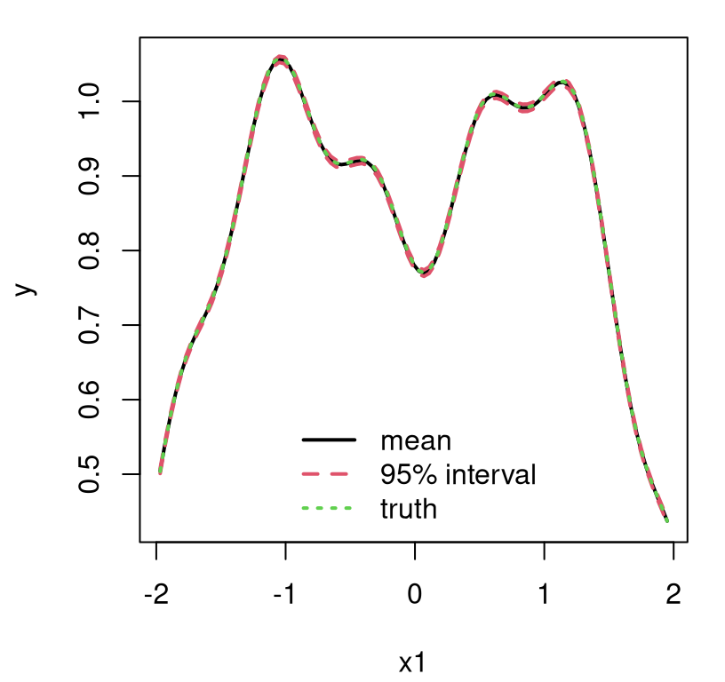
FIGURE 9.26: Slice \(x_2 = 0.51\) through Figure 9.25, augmented with predictive interval and true response.
What do we see? Prediction is accurate; had the green-dotted truth line been plotted first, with black mean coming after, the black would’ve completely covered the green, rendering it invisible. Error bars are very tight on the scale of the response; again, had black come after red we’d barely see red peeking out around black. Despite no continuity being enforced – calculations at nearby locations are independent and potentially occur in parallel – the resulting surface looks smooth to the eye.
What don’t we see? Accuracy, despite generally being high, is not uniform. Consider discrepancy with the truth, measured out-of-sample.
Figure 9.27 uses the same slice as above. We’re over-predicting. Systematic pattern and persistent positive bias is evident, although extremely small, judging by the scale of the \(y\)-axis.

FIGURE 9.27: Illustrating bias through differences between predictions and truth in the slice from Figure 9.26.
Remember that we’re using a zero-mean GP. Evidently in this slice, mean reversion is pulling us up a little too far, away from the training data and consequently away from the true response at these testing locations. Having an explanation helps, but it’s still unsatisfying to be leaving systematic predictive potential on the table. Also notice the lack of smoothness in the discrepancy surface. Training and testing responses are both smooth (and observed without noise), so it must be that the predictor – the LAGP surrogate – is not smooth. In fact it’s discontinuous, but on a small scale and not everywhere. Nearby predictive locations eventually share the same subdesign (as \(x' \rightarrow x\)) and thus inherit GP smoothness properties on a fine local scale.
Focusing on patterns evident in the bias plotted in Figure 9.27, what limits LAGP’s dynamic ability? Why does it leave such strong signal in the residuals? Considering the density of the input design in 2d, perhaps the fit is not flexible enough to characterize fast-moving changes in input–output relationships. Although an approximation, the local nature of modeling means that, from a global perspective, the predictor is more flexible than a full-\(N\) stationary GP predictor. So we can rest assured that an ordinary full GP wouldn’t fare any better in this regard, assuming the calculations were computationally tractable. Statistically independent fits in space, across elements of a vast predictive grid, lends aGP a degree of nonstationarity. By default, the laGP calls inside aGP go beyond that by learning separate \(\hat{\theta}_n(x)\) local to each \(x \in \mathcal{X}\) by maximizing local likelihoods.
In fact local lengthscales vary spatially, and relatively smoothly. Figure 9.28 plots \(\hat{\theta}_n(x)\) as \(x\) varies along our 1d slice. A loess smoothed alternative is overlayed in dashed-red.
plot(XX[zs,1], P.alc$mle$d[zs], type="l", lwd=2, xlab="x1",
  ylab="thetahat(x)")
df <- data.frame(y=log(P.alc$mle$d), XX)
lo <- loess(y ~ ., data=df, span=0.01)
lines(XX[zs,1], exp(lo$fitted)[zs], col=2, lty=2, lwd=2)
legend("topleft", "loess smoothed", col=2, lty=2, lwd=2, bty="n")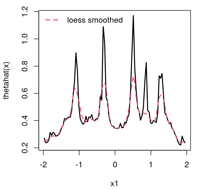
Spatial signal in rate of decay of inverse exponentiated squared Euclidean distance-based correlation is distinct in Figure 9.28, but the pattern doesn’t perfectly align with spatial bias along the slice shown in Figure 9.26. Smoothing \(\hat{\theta}_n(x)\) may help downplay numerical instabilities, but can in general represent a problem just as computationally difficult as the original one: an implicitly large-\(N\) spatial regression. Exceptions arise when working with grids, which is not uncommon if predicting for the purpose of visualization. (In other words, the tail doesn’t necessarily wag the dog when smoothing over \(\hat{\theta}_n(x)\)’s spatially in \(x\).)
Although the spatial field is locally isotropic, tacitly assuming stationarity to a certain extent, globally characteristics are less constrained. Nevertheless, the extra degree of flexibility afforded by spatially varying \(\hat{\theta}_n(x)\) is not enough to entirely mitigate the small amount of bias we saw above. Several enhancements offer potential for improved performance. Perhaps the first, and most obvious, entails deploying an anisotropic/separable correlation structure. That’s a mere implementation detail, so hold that thought for a moment.
Another option is to put those \(\hat{\theta}_n(x)\) to better use. You see, the local subdesign process must start somewhere – condition on “known” quantities – and laGP utilizes a fixed \(\theta_0 \equiv\) d to that end. By default, aGP invokes a built-in function called darg to choose a d to use identically for all \(x \in \mathcal{X} \equiv\) XX. Alternatively, a two-stage scheme, re-designing \(X_n(x) \mid \hat{\theta}_n(x)\), could help soften the influence of that ultimately arbitrary initialization. Below, subdesign search is based on the smoothed lengthscales from the first stage.
Basically, we’re redoing the whole local analysis, globally over all \(x \in \mathcal{X}\), but with a lengthscale unique to \(x\) and thus a subdesign tailored to dynamics nearby \(x\). Previously only the topology of the global design \(X_N\) mattered nearby \(x\) to determine \(X_n(x)\). Now conditioning on \(\hat{\theta}_n(x)\) from an earlier run gets responses \(Y_n\) involved too. Comparing predictions from the first iteration to those from the second in terms of RMSE …
##         alc      alc2
## 1 0.0006453 0.0003154
… reveals a degree of improvement, albeit perhaps not by an impressive amount (a factor of around 2 in this case). Such a two-stage analysis offers consistent, if slight improvement across a large swath of examples. Yet that thinking represents the tip of an iceberg: there are lots of ways to prime the pump, as it were. Before we get to those, let’s transition to a more ambitious example. By going back to the borehole (§9.1.3) we’ll be able to draw comparisons to a wider range of alternatives, coming full circle to CSK. (Objects x and y are unchanged from our earlier borehole examples, but X, Y and XX must be rebuilt from those.)
The borehole example benefits from long lengthscales, so aGP calls below adjust the default maximum lengthscale upwards to twenty. As with the default nugget g=1e-4, darg’s are conservative, but hold that thought for a moment. Long lengthscales are likely to yield poorly conditioned covariance matrices. Below an ordinary aGP run is invoked first, followed by a run primed with lengthscales \(\hat{\theta}_n \equiv\) out1$mle$d.
out1 <- aGP(X, Y, XX, d=list(max=20), omp.threads=nth, verb=0)
out2 <- aGP(X, Y, XX, d=list(start=out1$mle$d, max=20),
  omp.threads=nth, verb=0)
Recall that we used pointwise proper scores to compare CSK methods. The table below collects new timing and score results, combining with those obtained earlier for CSKs.
times <- c(times, aGP=as.numeric(out1$time), aGP2=as.numeric(out2$time))
scores <- c(scores, aGP=scorep(YY, out1$mean, out1$var),
  aGP2=scorep(YY, out2$mean, out2$var))
rbind(times, scores)
## sparse99 dense sparse999 aGP aGP2
## times 3260.863 3104.909 404.793 5.2330 4.9930
## scores -1.918 -6.962 -2.105 -0.6593 -0.6294That aGP is faster than our earlier CSK calculations is an understatement; the factor of improvement on time is a whopping 623. Local surrogates are also quite a bit more accurate. Perhaps this is surprising because aGP, being based on many independent laGP fits, utilizes far less data to make predictions. That can translate into over-estimates of variance which is penalized by score. Since training and testing data are noise free, one might instead compare using Mahalanobis distance, as explained in §5.2.1 nearby Eqs. (5.6)–(5.7). However, aGP only provides point-wise variance, necessitating a Mahalanobis approximation like Nash–Sutcliffe efficiency or out-of-sample \(R^2\). The curious reader may wish to update our comparison with those values, or consult the original G&A paper.
Now back to that separable lengthscale “implementation detail”. We’re able to beat CSK on two fronts, in time and score, with an isotropic correlation function. But CSK had the benefit of learning decay of correlation (and sparsity) in a coordinate-wise fashion. A function aGPsep, which is the separable analog of aGP, estimates separate lengthscales \(\theta_k(x)\) for each coordinate \(k=1,\dots,m\).
Using separable lengthscales represents a bigger implementation feat than at first it may seem, requiring an additional four thousand lines of C and R code in laGP. Working with a higher dimensional hyperparameter space, gradients, etc., demands extra scaffolding. One particular challenge centers around R’s built-in BFGS solver which, due to an antique implementation utilizing static variables, is not thread safe. Parallelization with OpenMP requires an intricate blocking mechanism to ensure that threaded BFGS calculations for \(\hat{\theta}_n(x)\) and \(\hat{\theta}_n(x')\) don’t interfere with one another. In the simpler scalar \(\theta\) setting laGP is able to avoid BFGS via R’s optimize (rather than optim) back-end.
Augmenting our table, notice below that utilizing separable lengthscales results in a similarly speedy execution, but yields substantially more accurate prediction.
times <- c(times, aGPs=as.numeric(outs$time))
scores <- c(scores, aGPs=scorep(YY, outs$mean, outs$var))
rbind(times, scores)
## sparse99 dense sparse999 aGP aGP2 aGPs
## times 3260.863 3104.909 404.793 5.2330 4.9930 5.39600
## scores -1.918 -6.962 -2.105 -0.6593 -0.6294 0.02829A second pass, priming a new aGPsep run with \(\hat{\theta}_n\)’s, offers slight improvements. Even better results may be obtained by taking a step back for more global perspective.
9.3.4 Global/local multi-resolution effect
Surely something is lost on this local approach to GP approximation. Kaufman et al. astutely observed that, especially when inducing sparsity in the covariance structure, it can be important to “put something global back in”. Recall that they partition modeling between trend (global/nonstationary) and residual (local/stationary), with the former being basis-expanded linear and the latter being spatial. That’s not easily mapped to the LAGP setup, which is the other way around: the local part is where the nonstationary effect comes in.
Towards an appropriate analog in the LAGP world, consider not a partition between trend and residual, but rather between lengthscales: global and local. Y. Liu (2014) showed that a “consistent” estimator of global (separable) lengthscale can be estimated through more manageably sized random data subsets if those subsets are generated with a block-bootstrap Latin hypercube sampling (BLHS) scheme. Also see Zhao, Amemiya, and Hung (2018). Rather than dig much under the surface of what Liu meant by “consistent”, instead let’s take it as “similar to what you’d get by maximizing the full data log likelihood”, i.e., the MLE. Basically, you don’t need to directly manipulate training data from a big design to estimate the lengthscale you would get from the big design. Now lengthscale hyperparameter estimates aren’t particularly useful on their own. A missing ingredient in that work is obtaining predictions, given those lengthscales, comparable to ones that would’ve been obtained from the big design. Those would still require big-matrix decomposition.
The idea is to convert global lengthscales into local subdesigns, subsequent local refinement of lengthscale, and ultimately tractable and accurate prediction. Here we take Liu’s BLHS as inspiration and use a simpler random subset analog. A random subset could not guarantee a similar distribution of pairwise distances compared to the original. From that perspective, BLHS accomplishes a feat akin to betadist designs introduced in §6.2.3, but for subdesign. See Sun, Gramacy, Haaland, Lawrence, et al. (2019) for more detail on BLHS, an implementation, and an empirical illustration of why it’s better than simple random subsampling, which nevertheless works very well as a quick-and-dirty alternative. A homework exercise in §9.4 invites readers to entertain a blhs (from laGP) variation of the following.
Consider a random 1000-sized subset in our running borehole example.
tic <- proc.time()[3]
nsub <- 1000
d2 <- darg(list(mle=TRUE, max=100), X)
subs <- sample(1:nrow(X), nsub, replace=FALSE)
gpsi <- newGPsep(X[subs,], Y[subs], rep(d2$start, m), g=1/1000, dK=TRUE)
that <- mleGPsep(gpsi, tmin=d2$min, tmax=d2$max, ab=d2$ab, maxit=200)
psub <- predGPsep(gpsi, XX, lite=TRUE)
deleteGPsep(gpsi)
toc <- as.numeric(proc.time()[3] - tic)
that$d
## [1] 0.4484 34.6612 36.4536 5.9560 31.9247 5.7086 2.3491 11.5727Values \(\hat{\theta}^{(g)} \equiv\) that quoted above don’t matter in and of themselves, but there they are. We can repeat that a bunch of times, in a bootstrap-like fashion, but that’s overkill. As a sanity check, observe that global random subset GP prediction is pretty good on its own, because the response is super smooth and pretty stationary.
times <- c(times, sub=toc)
scores <- c(scores, sub=scorep(YY, psub$mean, psub$s2))
rbind(times, scores)
## sparse99 dense sparse999 aGP aGP2 aGPs sub
## times 3260.863 3104.909 404.793 5.2330 4.9930 5.39600 113.3180
## scores -1.918 -6.962 -2.105 -0.6593 -0.6294 0.02829 0.6386In fact, that result almost makes you wonder what was going on with CSK. All that sparsity-inducing structure and it’d have been sufficient (even better) to take a random subset and run with that, in a fraction of the time. Subset-based GP surrogates even beat laGP, but at the expense of greater computation. Keep in mind this is a small example, and in particular that \(n_{\mathrm{sub}}=1000\) is a sizable portion of the total, \(N=4000\). It’s easy to engineer much larger-\(N\) examples where laGP is the only viable option in terms of accuracy per unit flop. The real power comes from combining global and local estimates.
A trick from Sun, Gramacy, Haaland, Lawrence, et al. (2019) is to use estimated global lengthscales \(\hat{\theta}^{(g)}\) to pre-scale inputs \(X_N\), and any testing locations \(\mathcal{X}\), so that afterwards the effective global lengthscales are 1. Careful, \(\theta\)-values modulate squared distance, so a square root must be taken before applying these back on the original scale of \(X_N\).
scale <- sqrt(that$d)
Xs <- X
XXs <- XX
for(j in 1:ncol(Xs)) {
  Xs[,j] <- Xs[,j]/scale[j]
  XXs[,j] <- XXs[,j]/scale[j]
}
Next fit LAGPs on these scaled inputs, stretching and compressing the input space, achieving a “multi-resolution effect”. With scaled inputs, an initial setting of d=1 makes sense. Otherwise the call below is the same as our aGP above. Notice that Y-values are the same as before. We’re not modeling a residual obtained from the “sub”-predictor, although we could. Local structure is isotropic (via aGP), but we could similarly do separable (via aGPsep). Both have been done before – even together – with success. The LAGP comparator included in a competition summarized by Heaton et al. (2018) was set up in that way, using aGPsep on residuals and pre-scaled inputs obtained from a random subset-trained GP predictor.
Before making yet another table with one new column, how about we do one more thing first (for two more columns instead)? The default nugget value in laGP/aGP is too large for most deterministic computer experiment applications. It was chosen conservatively so new users don’t get frustrated by inscrutable error messages. But we can safely dial it way down for this borehole example.
Table 9.2 finishes off the comparison with a prettier presentation, including the two new columns.
times <- c(times, aGPsm=as.numeric(out3$time),
  aGPsmg=as.numeric(out4$time))
scores <- c(scores, aGPsm=scorep(YY, out3$mean, out3$var),
  aGPsmg=scorep(YY, out4$mean, out4$var))
kable(t(rbind(times, scores)), digits=3,
caption="Comparing CSK and LAGP.")| times | scores | |
|---|---|---|
| sparse99 | 3260.863 | -1.918 |
| dense | 3104.909 | -6.962 |
| sparse999 | 404.793 | -2.105 |
| aGP | 5.233 | -0.659 |
| aGP2 | 4.993 | -0.629 |
| aGPs | 5.396 | 0.028 |
| sub | 113.318 | 0.639 |
| aGPsm | 5.057 | 1.027 |
| aGPsmg | 5.004 | 5.224 |
Wow, that’s lots better without lots more time! Technically, some of the times in the table above should incorporate time accrued by the earlier calculations they condition on. For example, a full accounting of compute times for aGPsm and aGPsmg would be 5 seconds longer. A caveat is that global random subset-based GP training of \(\hat{\theta}^{(g)}\) represents a fixed startup cost no matter how large the predictive set \(\mathcal{X}\) is.
9.3.5 Details and variations
Before turning to more realistic examples, including our motivating satellite drag application from §2.3 and CRASH calibration from §2.2, let’s codify LAGP algorithmically. Then I shall introduce some of the rather newer variations developed in order to support those challenging applications.
Algorithm
Pseudocode below details aGPsep, although its application with a singleton \(\mathcal{X} = \{x\}\), skipping Steps 1 and 3 (focusing only on 2), provides the essence of laGPsep. Local approximate GP regression at \(x\) is deployed as a subroutine applied identically over elements of a vast predictive set \(\mathcal{X}\). Isotropic aGP/laGP arise as trivial simplifications. The pseudocode is agnostic to a choice of active learning heuristic \(J(\cdot, \cdot)\) and covariance kernel \(K(\cdot, \cdot)\) except that the latter be distance-based as NNs are used in several places, e.g., as a means of priming and of short-cutting unnecessarily huge exhaustive searches through pre-selection of nearby candidates.
Algorithm 9.1: (Local) Approximate GP Regression
Assume criterion \(J(x_{j+1}, x; \theta)\), e.g., MSPE (9.2) or ALC, on distance-based covariance through hyperparameters \(\theta\) which are vectorized below; any priors/restrictions on \(\theta\) may be encoded through a log posterior/penalty addendum to GP log likelihood \(\ell(\theta ; D)\).
Require large-\(N\) training data \(D_N = (X_N, Y_N)\) and predictive/testing set \(\mathcal{X}\) which might be singleton \(\mathcal{X} = \{x\}\); local design size \(n \ll N\) with NN init size \(n_0 < n\) and NN search window size \(n \leq N' \ll N\).
Then
Optional multi-resolution modeling: additionally require subset size \(n < n_{\mathrm{sub}} \ll N\) and solve for global MLE hyperparameters; otherwise require initial \(\theta_0\) and set \(\theta \leftarrow \theta_0\).
- Draw \(n\) indices \(I_n \subset \{1,\dots,N\}\) without replacement and form global data subset \(D_n = (X_n, Y_n)\) where \(X_n = X_N[I_n,:]\) and \(Y_n = Y_N[I_n]\)
- Calculate \(\hat{\theta}^{(g)} = \mathrm{argmin}_\theta - \ell(\theta)\).
- Scale training and testing inputs:
\[ X_N[:,k] \leftarrow X_N[:,k] \Big{/} \sqrt{\hat{\theta}^{(g)}_k} \quad\mbox{and}\quad \mathcal{X}[:,k] \leftarrow \mathcal{X}[:,k] \Big{/} \sqrt{\hat{\theta}^{(g)}_k}, \quad \mbox{for } k=1,\dots,m. \]
- Set \(\theta \leftarrow 1\).
(Parallel) For each predictive location \(x \in \mathcal{X}\) calculate GP surrogate with data subset \(D_n(x)\).
- Build candidate set \(X^{\mathrm{cand}}_{N'}(x)\) of \(N'\) NNs in \(X_N\) to \(x\).
- Initialize \(X_{n_0}(x)\) with \(n_0\) nearest \(X^{\mathrm{cand}}_{N'}(x)\) to \(x\) and remove these from the candidate set, yielding \(X^{\mathrm{cand}}_{N'-n_0} (x)\).
- For \(j={n_0},\dots,n-1\), optimize criterion \(J\) to select
\[ x_{j+1} = \mathrm{argmin}_{x' \in X^{\mathrm{cand}}_{N'-j}} J(x', x; \theta) \quad \mbox{(exhaustively, approximately, in parallel).} \]
Update \(X_{j+1}(x) \leftarrow X_n \cup \{x_{j+1}\}\) and \(X^{\mathrm{cand}}_{N'-j-1}(x) \leftarrow X^{\mathrm{cand}}_{N'-j}(x) \setminus x_{j}\).
- Pair \(X_n(x)\) with \(Y_n\)-values to form local data \(D_n(x)\).
- Optionally update hyperparameters \(\theta \leftarrow \hat{\theta}_n(x)\) where
\[ \hat{\theta}_n(x) = \mathrm{argmin}_\theta - \ell(\theta; D_n(x)). \]
- Record predictions, e.g., pointwise means and variances (5.2) given \(\theta\) and \(D_n(x)\).
End For
- Optionally repeat Step 2 with \(\theta \leftarrow \hat{\theta}_n(x)\)-values, separately for each \(x\), potentially after smoothing.
Return predictions on \(\mathcal{X}\), e.g., as \(|\mathcal{X}| \times 2\) matrix of means and variances.
Several details, caveats and variations are worth explaining. Implementation in the laGP package calculates Student-\(t\) predictive equations under a reference prior for local scale parameter \(\tau^2\). Consequently, an additional degrees-of-freedom parameter is returned. Optionally, when Xi.ret=TRUE an \(|\mathcal{X}| \times n\) matrix of indices into \(X_N\) is returned to enable rebuilding of local designs and GP surrogates. Local MLE calculations (Step 2e) can be turned off with modifications to the d argument; incorporation of nuggets is facilitated by modifications to the default g argument. Only ALC is fully implemented by all variations: separable, isotropic, and otherwise. MSPE and Fisher information (FI) are provided as options for isotropic implementations only. Fully NN local approximation, which is accommodated by specifying \(n_0 = n\), could skip many of the lettered sub-steps of Step 2 in the algorithm. These are superfluous as NN calculation is not influenced by hyperparameters \(\theta\).
Step 1, creating a multi-resolution effect through pre-estimation of global lengthscale, assumes random subsampling; a BLHS alternative is similar, but would require an additional for loop. See blhs in the package documentation for more detail on this variation. Working with residuals from a global subset predictor (Heaton et al. 2018) is a potential variation that may be worth exploring. Step 2 may be SMP parallelized (on a single multi-core compute node) through the omp.threads argument to aGP/aGPsep. For distributed parallelization over the nodes of a cluster, see aGP.parallel. At this time there’s no aGPsep.parallel analog although a bespoke translation would be rather straightforward.
Step 2, implementing laGP/laGPsep local subdesign search as a subroutine, is initialized with start \(\equiv n_0 = 6\) NNs by default. Smaller start is not recommended on numerical stability grounds. Remaining local design selections, up to end \(\equiv n=50\), follow the greedy search criterion optimized in Step 2c. Rather than search over all \(X_N \setminus X_j(x)\), which might be an enormous set, Algorithm 9.1 utilizes local candidates \(X^{\mathrm{cand}}_{N'}(x)\) of \(N'\) NNs to \(x\). The number close \(\equiv N'\) of such candidates offers a compromise between full enumeration and an more limited approximate search. Package default close=1000 yields identical results compared to more exhaustive alternatives on a wealth of benchmark problems. Choosing \(N' = n\) would facilitate a clumsy reduction to fully NN local approximation.
Several alternative Step 2c implementations offer potential for further speedups from shortcuts under ALC. Providing method="alcray" replaces iteration over candidates with a 1d line search over rays emanating from \(x\) (Gramacy and Haaland 2016), with solutions snapped back to candidates. Derivatives offer another way to replace discrete with continuous search. Sun, Gramacy, Haaland, Lawrence, et al. (2019) provide details, with implementation as method="alcopt". In both cases the number of candidates \(N'\), to which continuous solutions are snapped, can safely be increased without taking a substantial computational hit. The laGP package automatically uses close=10000 for such cases. Gramacy, Niemi, and Weiss (2014) describe an exhaustive GPU-based search implemented in CUDA. Arguments including num.gpus, parallel="gpu", and alc.gpu support this interface, however special compilation of the original sources is required to enable these features. Speedups up to a factor of seventy have been observed in benchmarking exercises.
Finally, Step 3 provides the option of multiple passes through local design with refinements of hyperparameterization \(\hat{\theta}_n(x)\) learned in earlier stages. One re-pass can yield minor improvements in terms of predictive accuracy; more re-passes are not usually beneficial. When stretching and compressing inputs with globally estimated lengthscales \(\hat{\theta}^{(g)}\) from Step 1, re-passes offer limited additional benefit. (That is, typically one would not engage both of Steps 1 and 3 simultaneously.)
Joint path sampling
A downside of Algorithm 9.1 – equations furnished by aGP/aGPsep, or cluster analog aGP.parallel – is that predictive summaries are point-wise. A consequence of statistical independence, from which parallelization advantages stem, is a lack of predictive covariance across \(\mathcal{X} \equiv\) XX. Sun, Gramacy, Haaland, Lawrence, et al. (2019) describe how to extend LAGP to sets of points, which they call joint path sampling, motivated by a desire for joint predictive equations along a trajectory of orbits in their/our motivating satellite drag application (§2.3).
Consider a fixed, discrete and finite set of input locations \(W \subset \mathcal{X}\). A natural extension of the ALC criterion, the essence of which is reduction in variance \(v_j(x) - v_{j+1}(x)\), is
\[ \begin{aligned} &v_j(W)- v_{j+1}(W) = \frac{1}{|W|}\sum_{w \in W} \left\{v_j(w)-v_{j+1}(w)\right\}, \\ &\!= \frac{1}{|W|}\sum_{w \in W} \left\{ k_j^\top(w)G_j(x_{j+1})v_j(x_{j+1})k_j(w) \!+\! 2k_j^\top(w)g_j(x_{j+1})K(x_{j+1}, w) \!+\! \frac{K(x_{j+1}, w)^2 }{v_j(x_{j+1})} \right\}. \nonumber \end{aligned} \]
Notation here, including \(g_j\) and \(G_j\), etc., is borrowed from partitioned inverse-based updating equations (6.8) from §6.3. Observe that \(v_j(W)- v_{j+1}(W)\) is a scalar, measuring average reduction in predictive variance over \(W\). We wish to maximize over this criterion to greedily determine new \(x_{j+1}\) and augment local design \(X_j(W)\). Otherwise the setup is the same as \(X_n(x)\) with ALC, which arises as a special case under the degenerate path \(W = \{x\}\).
To illustrate, consider again Herbie’s tooth in 2d. Whenever you provide a set of reference locations to laGP/laGPsep, via Xref comprised of multiple rows, a joint path ALC criterion is automatically engaged. Joint path sampling is not implemented in the package for other criteria, \(J\), like MSPE. Code below recreates training data from earlier and designs a path \(W\) in 2d.
x <- seq(-2, 2, by=0.02)
X <- as.matrix(expand.grid(x, x))
Y <- herbtooth(X)
wx <- seq(-0.85, 0.45, length=100)
W <- cbind(wx - 0.75, wx^3 + 0.51)
Next, three variations on joint path sampling are entertained. The first is based on ALC. When using candidates \(X^{\mathrm{cand}}_{N'}(W)\) to shortcut local search it makes sense to allow \(N'\) to grow with the number of points (or length) of the path, \(|W|\). The second is NN: ignoring \(J\) and gathering samples based on nearest neighbors calculated in terms of aggregated Euclidean distance for all elements of \(W\). No candidates are required for this comparator. The third one approximates the first using derivative-based/continuous search (Sun, Gramacy, Haaland, Lawrence, et al. 2019), with snaps back to \(X^{\mathrm{cand}}_{N'}(W)\).
p.alc <- laGPsep(W, 6, 100, X, Y, close=10000, lite=FALSE)
p.nn <- laGPsep(W, 6, 100, X, Y, method="nn", close=10000, lite=FALSE)
p.alcopt <- laGPsep(W, 6, 100, X, Y, method="alcopt", lite=FALSE)
Providing lite=FALSE causes full predictive covariance matrices (5.3) to be returned. Visuals for these local joint path designs follow in Figure 9.29. Points selected by ALC are indicated as red open circles and denoted as “ALC-ex”. Suffix “-ex” reminds us that they’re based on exhaustive, discrete search. Analogous ones from NN (green diamonds) and derivative-based optimization (blue diamonds/“ALC-opt”) have been shifted down-right and up-left, respectively, to ease visualization. Path \(W\), in all three cases (shifted as appropriate), is shown as a solid black line.
plot(W, type="l", xlab="x1", ylab="x2", xlim=c(-2.25,0),
  ylim=c(-0.75,1.25), lwd=2)
points(X[p.alc$Xi,], col=2, cex=0.6)
lines(W[,1] + 0.25, W[,2] - 0.25, lwd=2)
points(X[p.nn$Xi,1] + 0.25, X[p.nn$Xi,2] - 0.25, pch=22, col=3, cex=0.6)
lines(W[,1] - 0.25, W[,2] + 0.25, lwd=2)
points(X[p.alcopt$Xi,1] - 0.25, X[p.alcopt$Xi,2] + 0.25, pch=23,
  col=4, cex=0.6)
legend("bottomright", c("ALC-opt", "ALC-ex", "NN"),
  pch=c(22, 21, 23), col=c(4, 2, 3))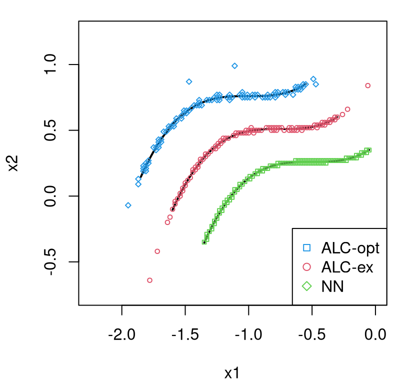
FIGURE 9.29: Joint local design along a path of predictive/reference locations under three criteria. Two paths are shifted from the original (middle) to ease visualization.
Observe how “ALC-ex” sacrifices some NNs for satellite points, primarily selected along rays emanating from the ends of the line \(W\). Some are quite far out. Derivative-based search, exemplified by “ALC-opt”, exhibits similar behavior but to a lesser extent. Instead it prefers satellite points off the middle of \(W\), which are likely inferior. Value in “ALC-opt” is primarily computational.
##    alc.elapsed alcopt.elapsed     nn.elapsed
##         11.016          0.227          0.059
Assessing these comparators out-of-sample would only be fair upon averaging over representative, but random, such \(W\). See randLine in the package. Sun et al. provide several such comparisons, including pointwise benchmarks. To summarize the outcome of those experiments: ALC-ex is the most accurate but also the slowest; NN is the fastest but least accurate. ALC-opt offers a nice compromise. As a testament to the value of joint path sampling, Figure 9.30 shows samples from the joint predictive distribution (5.3) provided by “ALC-ex”.
YY <- rmvnorm(100, p.alc$mean, p.alc$Sigma)
matplot(wx, t(YY), col="gray", type="l", lty=1,
  xlab="Indices wx of W", ylab="Y(W)")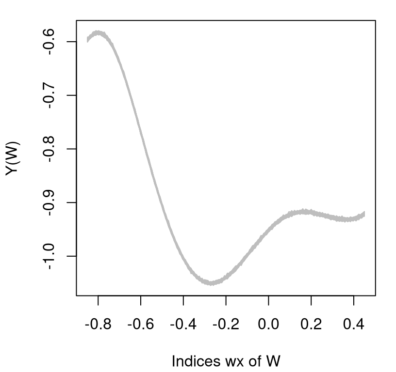
FIGURE 9.30: Full-covariance-based draws from the posterior predictive distribution along the local path from Figure 9.29.
Such samples would not be possible with an ordinary, pointwise (aGP/aGPsep) alternative. Note that although this example featured a connected \(W\), sampled discretely on a grid, the joint path sampling methodology, and its implementation in laGP/laGPsep, is applicable to any Xref \(\equiv W\) characterized as a discrete set of points and stored in a matrix. Recall that we looked at a similar setting in the context of reference-based IMSPE design in §6.1.2.
That concludes our methodological description and demonstration of LAGP surrogate modeling. For further examples, consult package documentation or see Gramacy (2016), which is also available as vignette("laGP") with the package. We turn now to two motivating applications where LAGP methods excel: large-scale satellite drag emulation (§2.3) and Kennedy and O’Hagan (KOH) style modularized calibration (§8.1.2) of radiative shock hydrodynamics computer simulations and field measurements (§2.2).
9.3.6 Two applications
Satellite drag
Let’s revisit the Hubble Space Telescope (HST) atmospheric drag simulations introduced in §2.3. Recall that the goal was to be able to predict drag coefficients (our response), globally in low Earth orbit (LEO), to within 1% root mean-squared percentage error (RMSPE). In §2.3 we restricted our analysis to a small training dataset with limited ranges of yaw and pitch angles. Here data from a larger simulation campaign is entertained over the full range of those angles. There are eight inputs, including HST’s panel angle, and supplementary material linked from the book web page contains files with 2 million runs obtained on LHS designs, separately for each chemical species (O, O\(_2\), N, N\(_2\), He, H). Our focus here will be on helium (He) runs, one of the harder species, whose design is built as two separate 1 million-sized LHSs.
Consider the first 1-million run LHS only.
## [1] 1000000Inputs are in natural units, so begin by coding these to the unit cube.
m <- ncol(hstHe) - 1
X <- hstHe[,1:m]
Y <- hstHe[,m+1]
maxX <- apply(X, 2, max)
minX <- apply(X, 2, min)
for(j in 1:ncol(X)) {
  X[,j] <- X[,j] - minX[j]
  X[,j] <- X[,j]/(maxX[j] - minX[j])
}
range(Y)
## [1] 0.3961 9.1920The range of output Y-values is relatively tame, so no need to re-scale these. It can help to center them, so that the mean-zero assumption in our (local approximate) GPs is not too egregiously violated, but that’s not required to get good results in this exercise. Sun, Gramacy, Haaland, Lawrence, et al. (2019) considered ten-fold CV on these data, and similarly for the other five species.
cv.folds <- function (n, folds=10)
  split(sample(1:n), rep(1:folds, length=n))
f <- cv.folds(nrow(X))
Our illustration here repeats one such random fold. Completing with the other nine folds is easily automated with a for(i in 1:length(f)) loop wrapped around the chunks of code entertained below.
i <- 1 ## potentially replace with for(i in 1:length(f))) { ...
o <- f[[i]]
Xtest <- X[o,]
Xtrain <- X[-o,]
Ytest <- Y[o]
Ytrain <- Y[-o]
c(test=length(Ytest), train=length(Ytrain))
## test train
## 100000 900000Using these data, the first inferential step is to fit a random subset GP. That simple surrogate serves as a benchmark on its own, and as the basis of a multi-resolution global/local lengthscale approach (§9.3.4). All together, the plan is to entertain three comparators: global subset GP, local approximate GP, and multi-resolution local/global approximate GP. Recall that drag simulations are not deterministic. They’re the outcome of a Monte Carlo (MC) solver called tpm. A large MC size was used to generate these data, so noise on outputs is quite low. I’ve hard-coded a small, but nontrivial nugget \(g=10^{-3}\) below. The curious reader may wish to try a (e.g., \(10\times\)) smaller nugget here. It doesn’t help, but it doesn’t hurt either. Out-of-sample mean accuracy results in this example are not much effected by the nugget as long as \(g\) is chosen to be reasonably small on the scale of range(Y).
da.orig <- darg(list(mle=TRUE), Xtrain, samp.size=10000)
sub <- sample(1:nrow(Xtrain), 1000, replace=FALSE)
gpsi <- newGPsep(Xtrain[sub,], Ytrain[sub], d=0.1, g=1/1000, dK=TRUE)
mle <- mleGPsep(gpsi, tmin=da.orig$min, tmax=10*da.orig$max, ab=da.orig$ab)
psub <- predGPsep(gpsi, Xtest, lite=TRUE)
deleteGPsep(gpsi)
rmspe <- c(sub=sqrt(mean((100*(psub$mean - Ytest)/Ytest)^2)))
rmspe
## sub
## 11.4These results are similar to ones we obtained with a pilot exercise in §2.3: not even close to the 1% target. How about a separable local GP?
alcsep <- aGPsep(Xtrain, Ytrain, Xtest, d=da.orig, omp.threads=nth, verb=0)
rmspe <- c(rmspe, alc=sqrt(mean((100*(alcsep$mean - Ytest)/Ytest)^2)))
rmspe
## sub alc
## 11.398 5.829Much better, but not quite to 1%. Our final comparator is the global/local multi-resolution approximation based on local GPs applied to inputs stretched and compressed by the mle calculated on the subset above.
for(j in 1:ncol(Xtrain)) {
  Xtrain[,j] <- Xtrain[,j]/sqrt(mle$d[j])
  Xtest[,j] <- Xtest[,j]/sqrt(mle$d[j])
}
Before setting things running it helps to re-construct a default prior appropriate for scaled inputs.
Finally, fit locally on globally scaled inputs.
alcsep.s <- aGPsep(Xtrain, Ytrain, Xtest, d=da.s, omp.threads=nth, verb=0)
rmspe <- c(rmspe, alcs=sqrt(mean((100*(alcsep.s$mean - Ytest)/Ytest)^2)))
rmspe
## sub alc alcs
## 11.398 5.829 0.779Although results here are somewhat sensitive to the random CV fold, more often than not this local–global surrogate beats 1%. In addition to being more accurate, the multi-resolution fit is actually faster than its pure-local alternative.
##  alc.elapsed alcs.elapsed
##           55           43
This speedup, of about 22%, stems from two factors. One is that local MLE calculations for \(\hat{\theta}(x)\) require fewer iterations after scaling inputs and initializing search from d=1.
## better     x2
## 0.7943 0.2479
As you can see above, 79% of testing locations \(x \in \mathcal{X} \equiv\) Xtest required fewer BFGS iterations for the latter comparator, corresponding to the multi-resolution case, than for the former. About 25% of the time the latter was two times better. Fewer iterations means faster execution. It also means less OpenMP blocking to circumvent static variable shortcomings in R’s internal BFGS implementation, and thus higher engagement of running threads on idle cores. The first, alcsep run had 400% engagement (of a total 800%) on my 8-core machine; alcsep.s had about 500% thanks to lower latency in OpenMP blocking from faster lbfgsb calculations. Finally, a similar aGPsep run from an laGP package linked to Intel MKL R (and executed off-line of this Rmarkdown build) gets consistently above 700% because that latency is further reduced by fast matrix decompositions in local MLE calculations. Total runtime for alcsep.s is reduced from 43 down to about 21 minutes with MKL. That’s pretty amazing for 100 thousand predictions on 900 thousand training points.
How may even better results be obtained? Several ways: use more data (augmenting with the other 1 million LHS); use BLHS rather than random subsampling for estimating \(\hat{\theta}^{(g)}\); perform a second stage of local analysis, conditioned upon \(\hat{\theta}_n(x)\). Keen readers are encouraged to pursue these alternatives in a homework exercise combining all six pure-species predictors (i.e., H, N, N\(_2\), O, and O\(_2\) in addition to He, above) in order to obtain accurate ensemble predictors (§2.3.2) out-of-sample.
Large-scale calibration
Modularized KOH calibration from §8.1.2 relied on computer surrogate model predictions at a small number \(n_F\) of field data sites \(X_{n_F}\) paired with “promising” values of the calibration parameter \(u\). In other words, surrogate GP prediction is only required at a relatively small set of locations, determined on-line as optimization over \(u\) proceeds in search of \(\hat{u}\), regardless of the (potentially massive) size of the computer experiment \(N_M \gg n_F\). Local GPs couldn’t be more ideal for this situation, furnishing quick approximations to \(y^M(x, \cdot)\) nearby testing sites, e.g., for \(x \in X_{n_F}\) paired with \(u\)-values along a trajectory toward \(\hat{u}\). Algorithm 9.2 makes that explicit by re-defining Steps 1–2 of our earlier (full GP/agnostic surrogate) version in Algorithm 8.2 from §8.1.3.
Algorithm 9.2: LAGP-based Modifications to Modularized KOH Calibration via Optimization (Algorithm 8.2)
Assume and Require are unchanged except that laGP-based methods are used for surrogate modeling \(y^M(\cdot, \cdot)\).
Then
- Let \([X_{n_F}, u^\top]\) denote calibration-parameter augmented field data locations obtained by concatenating \(u^\top\) identically to each of \(n_F\) rows of field data inputs \(X_{n_F}\).
- Form the objective
obj(u)as follows:- Obtain surrogate predictive mean values \(\hat{Y}_{n_F}^{M|u} = \mu(X_{n_F}, u)\) from local surrogate \(\hat{y}^M(\cdot, u)\), e.g., via
aGP/aGPsepevaluations withXX\(\equiv [X_{n_F}, u^\top]\) and training dataX\(\equiv (X_{N_M}, U_{N_M})\) andY\(\equiv Y_{N_M}\). - – d. unchanged
- Obtain surrogate predictive mean values \(\hat{Y}_{n_F}^{M|u} = \mu(X_{n_F}, u)\) from local surrogate \(\hat{y}^M(\cdot, u)\), e.g., via
- Solve \(\hat{u} = \mathrm{argmin}_u -\)
obj\((u)\) with a derivative-free solver,- e.g.,
snomadrin thecrspackage for R.
- e.g.,
- unchanged
Return unchanged.
Several variations may be worth entertaining. LAGP surrogate fits, via aGP/aGPsep, could be enhanced with multi-resolution global/local or multi-pass local refinement of lengthscale. Steps 2b–d, which detail fitting discrepancy between computer model predictions and field data responses can utilize GP regression with a nugget, as favored in §8.1.3. Alternatively, something entirely different could be entertained, including a “nobias” alternative (§8.1.4). Local GPs only substitute for computer model surrogate. While they could equally be deployed for discrepancy, which might be helpful if \(n_F\) is also large, I’m not aware of any successful such applications in the literature.
It’s easy to overlook Step 3 in Algorithm 9.2 as an insignificant modification. It calls for derivative-free optimization (Larson, Menickelly, and Wild 2019) over \(u\), whereas in Algorithm 8.2 optim was recommended. The trouble here is the discrete nature of independent local design searches for \(\hat{y}^M(x_j^F, u)\), for each index \(j=1,\dots, n_F\) into \(X_{n_F}\). These ensure an objective (8.4), quoted here as
\[ p(u) \left[ \max_{\theta_b} p_b(\theta_b \mid D^{b}_{n_F}(u)) \right], \]
that’s not continuous in \(u\). Discontinuous objectives thwart derivative (BFGS) or continuity-based (Nelder-Mead) solvers, although some are more robust to such nuances than others. Gramacy et al. (2015) suggest mesh adaptive direct search [MADS; Audet and Dennis Jr (2006)] as implemented in NOMAD. An interface for R is furnished by subroutines in crs (Racine and Nie 2018) on CRAN.
As MADS is a local solver, NOMAD requires initialization. Gramacy et al. suggest choosing starting \(u^{(0)}\)-values from the best value(s) of the objective found on a small space-filling design. The laGP package contains several functions that automate the objective explained in Algorithm 9.2: fcalib is like calib from §8.1, returning - obj\((u)\) evaluations (in log space) for minimization; discrep.est is like bhat.fit; special cases for nobias calibration are also implemented. For more details see Section 4.2 of Gramacy (2016), or as vignette("laGP").
To illustrate, revisit the setup from exercise #2 in §8.3 with synthetic computer model
\[ y^M(x, u) = \left(1-e^{-\frac{1}{2x_2}}\right) \frac{1000 u_1 x_1^3 + 1900 x_1^2+2092 x_1+60}{100 u_2 x_1^3 + 500 x_1^2 + 4x_1+20}, \]
borrowed from Goh et al. (2013), but originally due to Bastos and O’Hagan (2009). Design inputs \(x\) and calibration parameters \(u\) are both unit two-dimensional, which eases visualization. An implementation in R is provided below.
M <- function(x, u)
 {
  x <- as.matrix(x)
  u <- as.matrix(u)
  out <- (1 - exp(-1/(2*x[,2])))
  out <- out*(1000*u[,1]*x[,1]^3 + 1900*x[,1]^2 + 2092*x[,1] + 60)
  out <- out/(100*u[,2]*x[,1]^3 + 500*x[,1]^2 + 4*x[,1] + 20)
  return(out)
 }
Again slightly simplifying from Goh et al. (2013), the field data are generated as
\[ \begin{aligned} y^F(x) &= y^M(x, u^\star) + b(x) + \varepsilon, \;\; \mbox{ where } \; b(x) = \frac{10x_1^2+4x_2^2}{50 x_1 x_2+10} \\ \mbox{ and } \; \varepsilon &\stackrel{\mathrm{iid}}{\sim} \mathcal{N}(0, 0.5^2), \end{aligned} \]
using \(u^\star=(0.2, 0.1)\). In R \(b(\cdot)\) may be implemented as follows.
bias <- function(x)
 {
  x <- as.matrix(x)
  out <- (10*x[,1]^2 + 4*x[,2]^2)/(50*x[,1]*x[,2] + 10)
  return(out)
 }
Compared to the homework, our example here will follow Gramacy et al. (2015) for a slightly bigger field experiment with \(n_F = 100\) runs formed of two replicates of 50-sized 2d LHS of \(x\)-values; and a much bigger simulation experiment with \(N_M = 10500\) runs comprised of a 4d LHS of size 10000 of \((x,u)\)-values, augmented with runs at the 50 unique field data sites \(x\) randomly paired with a 500-sized 2d LHS of \(u\)-values. Code immediately below generates the field experiment component of these data, where Zu holds intermediate computer model evaluations at \(u^\star\).
ny <- 50
X <- randomLHS(ny, 2)
u <- c(0.2, 0.1)
Zu <- M(X, matrix(u, nrow=1))
sd <- 0.5
reps <- 2
Y <- rep(Zu, reps) + rep(bias(X), reps) + rnorm(reps*length(Zu), sd=sd)
length(Y)
## [1] 100Next, the computer experiment component is designed and simulations are run with a Z object storing output \(Y_{N_M}\)-values.
nz <- 10000
XU <- randomLHS(nz, 4)
XU2 <- matrix(NA, nrow=10*ny, ncol=4)
for(i in 1:10) {
  I <- ((i-1)*ny + 1):(ny*i)
  XU2[I, 1:2] <- X
}
XU2[,3:4] <- randomLHS(10*ny, 2)
XU <- rbind(XU, XU2)
Z <- M(XU[,1:2], XU[,3:4])
length(Z)
## [1] 10500The following code chunk sets default priors and specifies details of the laGP-based surrogate and (full) GP bias.
Changing bias.est <- FALSE causes estimation of \(\hat{b}(\cdot)\) to be skipped. Instead only the level of noise between computer model and field data is estimated, setting up a nobias calibrator. The methods vector specifies the nature of search and number of passes through simulation data for local design and inference. We’ll be doing two passes of isotropic ALC local design search where the second pass is primed with \(\hat{\theta}_n(x)\)’s from the first one. The model is completed with a (log) prior density on calibration parameter \(u\), chosen to be independent Beta with mode in the middle of the space. This choice is made primarily to avoid boundary-focused \(\hat{u}\) as discussed in §8.1.5 and revisited in homework exercises.
Now evaluate the objective on a space-filling grid to search for good starting values for subsequent NOMAD optimization. Our “grid” is actually a maximin LHS (§4.3) focused away from the edges of the input space.
The for loop below collects objective evaluations on that “grid” through fcalib calls.
llinit <- rep(NA, nrow(uinit))
for(i in 1:nrow(uinit)) {
  llinit[i] <- fcalib(uinit[i,], XU, Z, X, Y, da, d, g, lprior,
    methods, NULL, bias.est, nth, verb=0)
}
Finally we’re ready to optimize. The snomadr interface allows a number of options to be passed to NOMAD. Those provided below have been found to work well in a number of laGP-based calibration examples. The NOMAD user guide can be consulted for more detail and information on further options.
library(crs)
imesh <- 0.1
opts <- list("MAX_BB_EVAL"=1000, "INITIAL_MESH_SIZE"=imesh,
  "MIN_POLL_SIZE"="r0.001", "DISPLAY_DEGREE"=0)
Unfortunately snomadr doesn’t provide any mechanism for saving progress information, which will be handy later for visualization. So fcalib has an optional save.global argument for specifying in which R environment (e.g., .GlobalEnv) to save such relevant information. R code below invokes snomadr on the best input(s) found on the starting grid, looping over them until a minimum number of NOMAD iterations has been reached. Usually just one pass through this outer loop is sufficient, i.e., using only the very best starting location. In situations where NOMAD may prematurely converge, having a backup starting location (or two) can be handy.
its <- 0
i <- 1
out <- NULL
o <- order(llinit)
while(its < 10) {
  outi <- snomadr(fcalib, 2, c(0,0), 0, x0=uinit[o[i],], lb=c(0,0),
    ub=c(1,1), opts=opts, XU=XU, Z=Z, X=X, Y=Y, da=da, d=d, g=g,
    methods=methods, M=NULL, verb=0, bias=bias.est, omp.threads=nth,
    uprior=lprior, save.global=.GlobalEnv)
    its <- its + outi$iterations
    if(is.null(out) || outi$objective < out$objective) out <- outi
    i <- i + 1
}
##
## iterations: 14
## time: 95What came out? Here’s some code that reads the fcalib.save object stored in .GlobalEnv to prepare a plot for the forthcoming figure. Objective (fcalib) evaluations from both grid and NOMAD optimization are combined and used as the basis of a reconstruction of a 2d surface in \(u\)-space.
Xp <- rbind(uinit, as.matrix(fcalib.save[,1:2]))
Zp <- c(-llinit, fcalib.save[,3])
wi <- which(!is.finite(Zp))
if(length(wi) > 0) {
  Xp <- Xp[-wi, ]
  Zp <- Zp[-wi]
}
library(akima)
surf <- interp(Xp[,1], Xp[,2], Zp, duplicate="mean")
u.hat <- out$solution
The interp command above, from akima (Akima et al. 2016) on CRAN, projects these “\(z\)” coordinates onto an “\(x\)–\(y\)” mesh used by image in Figure 9.31. Lighter/whiter colors correspond to higher (log) objective evaluations. The grid of initial runs is indicated by open circles; NOMAD evaluations are shown as green diamonds, and the best of those (\(\hat{u}\)) as a solitary blue diamond. The true data-generating value of the calibration parameter \(u^\star\) is indicated by an intersecting pair of horizontal and vertical dashed lines.
image(surf, xlab="u1", ylab="u2", col=heat.colors(128),
  xlim=c(0,1), ylim=c(0,1))
points(uinit)
points(fcalib.save[,1:2], col=3, pch=18)
points(u.hat[1], u.hat[2], col=4, pch=18)
abline(v=u[1], lty = 2)
abline(h=u[2], lty = 2)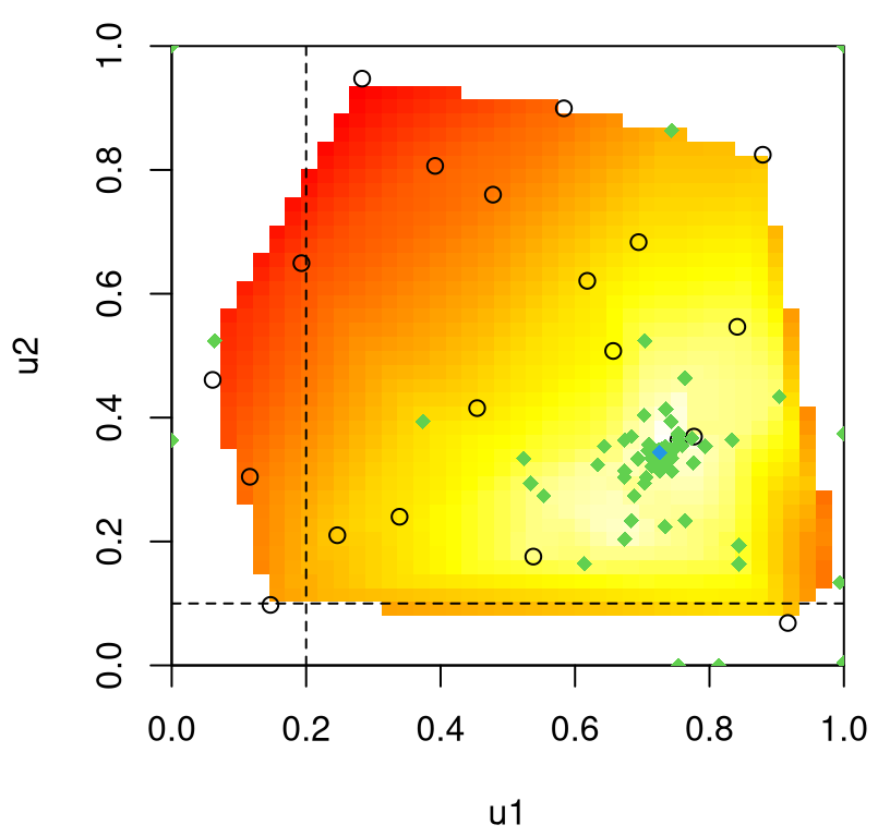
FIGURE 9.31: Log posterior surface for \(u\) built by linearly interpolating evaluations under an initial maximin LHS (open circles) and NOMAD evaluations (green diamonds). MAP estimate \(\hat{u}\) is indicated by a blue diamond. Cross-hairs show true \(u^\star\).
So true \(u^\star\) is far from the \(\hat{u}\) that we found. Indeed, the surface is fairly peaked around \(\hat{u}\), giving very little support to regions nearby the true value. Admittedly, very few \(u\)-evaluations were tried nearby \(u^\star\). It may be worth checking if our scheme missed an area of high likelihood.
obju <- fcalib(u, XU, Z, X, Y, da, d, g, lprior, methods, NULL, bias.est,
  nth, verb=0)
c(u.hat=out$objective, u.star=obju)
## u.hat u.star
## 127.4 131.4Nope: our \(\hat{u}\) is better than the true \(u^\star\). (Recall that fcalib is designed for minimization, so smaller is better.) Perhaps a better question is: which (\(\hat{u}\) or \(u^\star\)) leads to better prediction out-of-sample? Obtaining a predictor that can be used at new testing locations, the following code goes step-by-step through calls automated by fcalib.
Xu <- cbind(X, matrix(rep(u, ny), ncol=2, byrow=TRUE))
Mhat.u <- aGP.seq(XU, Z, Xu, da, methods, ncalib=2,
  omp.threads=nth, verb=0)
cmle.u <- discrep.est(X, Y, Mhat.u$mean, d, g, bias.est, FALSE)
cmle.u$ll <- cmle.u$ll + lprior(u)
-cmle.u$ll
## [1] 131.4The final line above serves as a sanity check that indeed that code duplicates the process behind fcalib: same as obju above. Entry cmle.u$gp holds the bias-correcting GP reference, which we shall use momentarily to make predictions. First, build up a testing set with computer model evaluations on 1000 new space-filling sites \(x\), all paired with true data-generating value \(u^\star\), followed by true discrepancy. No noise is added to these out-of-sample validation responses.
Now consider prediction and subsequent RMSE calculation with true \(u^\star\).
XXu <- cbind(XX, matrix(rep(u, nny), ncol=2, byrow=TRUE))
Mhat.oos.u <- aGP.seq(XU, Z, XXu, da, methods, ncalib=2,
  omp.threads=nth, verb=0)
YYm.pred.u <- predGP(cmle.u$gp, XX)
YY.pred.u <- YYm.pred.u$mean + Mhat.oos.u$mean
rmse.u <- sqrt(mean((YY.pred.u - YYtrue)^2))
deleteGP(cmle.u$gp)
For estimated \(\hat{u}\) we must first backtrack through what fcalib automated earlier and save surrogate predictions and estimated bias-corrections.
Xu <- cbind(X, matrix(rep(u.hat, ny), ncol=2, byrow=TRUE))
Mhat <- aGP.seq(XU, Z, Xu, da, methods, ncalib=2, omp.threads=nth, verb=0)
cmle <- discrep.est(X, Y, Mhat$mean, d, g, bias.est, FALSE)
cmle$ll <- cmle$ll + lprior(u.hat)
Here’s a sanity check that this gives the same objective evaluation as what came out of snomadr.
## [1] 127.4 127.4Finally, repeat what we did above with the true \(u^\star\) value, but with estimated \(\hat{u}\) instead.
XXu <- cbind(XX, matrix(rep(u.hat, nny), ncol=2, byrow=TRUE))
Mhat.oos <- aGP.seq(XU, Z, XXu, da, methods, ncalib=2,
  omp.threads=nth, verb=0)
YYm.pred <- predGP(cmle$gp, XX)
YY.pred <- YYm.pred$mean + Mhat.oos$mean
rmse <- sqrt(mean((YY.pred - YYtrue)^2))
deleteGP(cmle$gp)
How do these RMSEs compare?
##  u.hat      u
## 0.1177 0.1248
Indeed, our estimated \(\hat{u}\) version leads to better predictions too. Clearly there’s an identifiability issue – something other than the true data-generating parameter works better – in this supremely flexible calibration apparatus; but it does a good job of predicting. Other merits include that the framework is computationally thrifty. Although no timing results are quoted by the code above, this entire segment on large-scale laGP-based calibration takes but a few minutes to run. Our illustrative example was synthetic, but served to highlight many of the pertinent features of the methodology and its implementation. Porting that setup to the motivating CRASH data from §2.2 is rather straightforward. A homework exercise in §9.4 takes the reader through the details.
The core idea of tailoring GP prediction to the application goal, in a transductive fashion, is catching on as a means of gaining computational tractability and modeling fidelity. For example, Gul (2016) developed a so-called in situ emulator where the surrogate is tailored to a UQ task focused around a nominal input setting. J. Huang et al. (2020) develop a similar framework of on-site surrogates (OSSs) for a large-run (big \(N\)), large input dimension (\(m\)), computer model calibration problem. This is similar in spirit to laGP-based KOH calibration except that design of new computer model runs is incorporated directly into surrogate construction in lieu of sub-selecting points from an existing design.
To close out this chapter, it’s worth acknowledging that the methods described herein are at best representative and at worst barely scratch the surface of the state-of-the-art of thrifty surrogate modeling. Pace of development of new methodology for large-scale GP approximation is feverish. My goal was to provide some depth, but at the expense of clear bias toward methodology I know well. Nevertheless we covered all of the important pillars: sparsity, divide-and-conquer, parallel computing and hybridization (e.g., global and local). A downside to all of these approaches, but especially those leveraging divide-and-conquer, is that they sacrifice smoothness and force compromise to be struck between local/dynamic behavior and global/long range features. For situations where, for example, mean and variance evolve smoothly throughout the input space – a feature common to many modern stochastic computer model simulations – a different perspective is warranted.
9.4 Homework exercises
Exercises focusing primarily on tgp and laGP follow, in several cases circling back to motivating examples from Chapter 2 with a proper treatment.
#1: Sequential design with tgp
Revisit exercise #5 from §6.4, on sequential design for a nonstationary process, but this time using treed Gaussian processes. In particular, consider #5b with ALM and ALC heuristics under btgp, using any approximations or options you deem necessary for the method to be fast enough on your machine in order to complete the full exercise. Repeat multiple times (say thirty), report average RMSE-based progress and the distribution of final RMSEs measured on the full dataset. As in the original description of the problem, restrict yourself to the side output, and two-dimensional input spaces in the beta=2 slice. Make an explicit comparison between your new TGP-based results and those you previously obtained for the stationary GP (1) and manual 2-partition GP (2) in your solution to #5 from §6.4. For brownie points, extend the comparison to the full 3d input space.
#2: SARCOS robotics data
The SARCOS data features as a prime example in Rasmussen and Williams (2006). These data come pre-partitioned as a set of about 44 thousand training runs, and 4.4 thousand testing runs, both having twenty-one inputs and seven outputs. Consider here just the first of the seven outputs. For more details, see the link(s) above. MATLAB files storing these data have been converted to plain text and are linked here: train and test. Entertain the following comparators in terms of compute time (combining learning and prediction) and out-of-sample RMSE.
- NN-based local approximate GP (LAGP) with isotropic and separable alternatives (
aGP/aGPsepwithmethod=nn"), local design size \(n \equiv\)end=50(default) and \(n \equiv\)end=200; - ALC-based LAGP, both isotropic and separable (
aGP/aGPsepwith defaultmethod="alc"); - ALC-based LAGP with approximate ray search, both isotropic and separable (
aGP/aGPsepwithmethod="alcray"); - Separable GP trained on a random subsample of 1000 input–output pairs;
- Revisit #i–iii with inputs stretched and compressed by the MLE lengthscales from #iv for a multi-resolution effect (§9.3.4).
You should have a total of seventeen comparators. Code inputs for #i–iv into \([0,1]^{21}\), fix the nugget at \(g=1/1000000\) and use priors on the lengthscale built with darg using samp.size=10000. Base predictors for #v variations on scaled versions of coded inputs and appropriately modified priors. Provide visuals capturing time-versus-accuracy trade-offs, possibly on log scales.
#3: Ensemble satellite drag benchmarking
Revisit exercise #3 from §2.6 combining surrogates for pure-species simulations under a realistic mixture of chemical species in LEO, but this time use the big simulation sets over the entire range of pitch and yaw angles. Specifically, choose one of the following:
- HST via 2-million run (8d) LHS pure-species training sets, which may be found in
tpm-git/data/HST/hst[H,He,He2,N,N2,O,O2].dat, and ensemble testing set residing intpm-git/data/HST/hstEns.dat. Note that you’ll need to combineHeandHe2to obtain the full 2-million training runs for pure helium; - or GRACE via 1-million run (7d) LHS pure-species training sets residing in
tpm-git/data/GRACE/grace[H,He,He2,N,N2,O,O2].datand ensemble testing set which can be found intpm-git/data/GRACE/graceEns.dat.
Work with inputs coded to \([0,1]^m\). Subsequently stretch and compress those coded inputs using MLE lengthscales obtained from a surrogate fit to a 1000-sized random subset to achieve a multi-resolution effect (§9.3.4). Hint: When fitting a global subset GP to GRACE simulations, you might find it helpful to initialize MLE calculation for lengthscales with c(rep(1,5), 0.01, 0.1). Obtain predictions at coded and scaled ensemble inputs under the six multi-resolution global–local (§9.3.4) surrogates, and combine them by the appropriate weighted average (§2.3.2). Confirm that your out-of-sample RMSPE is below LANL’s 1% target. You may wish to compare your results to BLHS-based pre-scaling instead (§9.3.4), using the blhs function in laGP.
#4: CRASH calibration
Consider the radiative shock hydrodynamics (CRASH) example from §2.2, which is described as a calibration problem. There are nine design variables (\(x\)), two calibration parameters (\(u\)), two computer experiments with a combined five thousand or so runs, and a field data experiment with twenty observations. Combining the two computer experiments necessitates an expansion of the dataset vis-à-vis one of the calibration parameters, so that there are more like twenty thousand runs. That data setup is given in the code below.
## read in computer model runs
rs12 <- read.csv("crash/RS12_SLwithUnnormalizedInputs.csv")
rs13 <- read.csv("crash/RS13Minor_SLwithUnnormalizedInputs.csv")
## a correction
rs13$ElectronFluxLimiter <- 0.06

## read in the physical data
crash <- read.csv("crash/CRASHExpt_clean.csv")
## a correction
crash$BeThickness <- 21

## create expanded computer model data
sfmin <- rs13$EffectiveLaserEnergy/5000
sflen <- 10
rs13.sf <- matrix(NA, nrow=sflen*nrow(rs13), ncol=ncol(rs13)+2)
for(i in 1:sflen) {
  sfi <- sfmin + (1 - sfmin)*(i/sflen)
  rs13.sf[(i-1)*nrow(rs13) + (1:nrow(rs13)),] <-
    cbind(as.matrix(rs13), sfi, rs13$EffectiveLaserEnergy/sfi)
}
rs13.sf <- as.data.frame(rs13.sf)
names(rs13.sf) <- c(names(rs13), "EnergyScaleFactor", "LaserEnergy")

## merge the data.frames
rsboth <- rbind(rs12, rs13.sf[,names(rs12)])

## extract out Xs and Ys
XU.orig <- rsboth[,-which(names(rsboth) %in%
  c("FileNumber", "ShockLocation"))]
Z.orig <- rsboth$ShockLocation
X.orig <- crash[,names(XU.orig)[1:(ncol(XU.orig) - 2)]]
Y.orig <- crash$ShockLocation

## scale to coded outputs
minZ <- min(Z.orig)
maxZ <- max(Z.orig)
Z <- Z.orig - minZ
Z <- Z/(maxZ - minZ)
Y <- Y.orig - minZ
Y <- Y/(maxZ - minZ)

## scale to coded inputs
maxX <- apply(XU.orig, 2, max)
minX <- apply(XU.orig, 2, min)
XU <- XU.orig
X <- X.orig
for(j in 1:ncol(XU)) {
  XU[,j] <- XU[,j] - minX[j]
  XU[,j] <- XU[,j]/(maxX[j] - minX[j])
  if(j <= ncol(X)) {
    X[,j] <- X[,j] - minX[j]
    X[,j] <- X[,j]/(maxX[j] - minX[j])
  }
}
Your task is to use laGP to perform a computer model calibration on these data. Report on the estimate of \(\hat{u}\) that you obtained from a modularized KOH setup (estimate a bias correction; no need to entertain a nobias alternative). Finally, gather predictions at the following \(x\)-values: Be thick 21, laser energy 3800, Xe fill 1.15, tube diam 1150, taper length 500, nozzle length 500, aspect ratio 2, time 26. Note that this example is entertained in Gramacy et al. (2015), which you may use as guidance/inspiration. Although inputs and outputs are coded, report predictions, etc., back on the natural scale.
References
akima: Interpolation of Irregularly and Regularly Spaced Data. https://CRAN.R-project.org/package=akima.
Matrix: Sparse and Dense Matrix Classes and Methods. https://CRAN.R-project.org/package=Matrix.
randomForest: Breiman and Cutler’s Random Forests for Classification and Regression. https://CRAN.R-project.org/package=randomForest.
xgboost: Extreme Gradient Boosting. https://CRAN.R-project.org/package=xgboost.
BayesTree: Bayesian Additive Regression Trees. https://CRAN.R-project.org/package=BayesTree.
spBayes: Univariate and Multivariate Spatial-Temporal Modeling. https://CRAN.R-project.org/package=spBayes.
tgp: An R Package for Bayesian Nonstationary, Semiparametric Nonlinear Regression and Design by Treed Gaussian Process Models.” Journal of Statistical Software 19 (9): 6.
laGP: Large-Scale Spatial Modeling via Local Approximate Gaussian Processes in R.” Journal of Statistical Software 72 (1): 1–46.
laGP: Local Approximate Gaussian Process Regression. http://bobby.gramacy.com/r_packages/laGP.
tgp Version 2, an R Package for Treed Gaussian Process Models.” Journal of Statistical Software 33 (6): 1–48.
tgp: Bayesian Treed Gaussian Process Models. https://CRAN.R-project.org/package=tgp.
dynaTree: Dynamic Trees for Learning and Design. https://CRAN.R-project.org/package=dynaTree.
gbm: Generalized Boosted Regression Models. https://CRAN.R-project.org/package=gbm.
GpGp: Fast Gaussian Process Computation Using Vecchia’s Approximation. https://CRAN.R-project.org/package=GpGp.
BART: Bayesian Additive Regression Trees. https://CRAN.R-project.org/package=BART.
crs: Categorical Regression Splines. https://CRAN.R-project.org/package=crs.
gbm Package.” R package vignette: https://cran.r-project.org/web/packages/gbm/vignettes/gbm.pdf.