Chapter 6 Model-based Design for GPs
Chapter 4 offered a model-free perspective on design, choosing to spread out \(X_n\) where \(Y_n\) will be observed, with the aim of fitting a flexible nonlinear, nonparametric, but ultimately generic regression. Gaussian processes (GPs) were on our mind, but only as a notion. Now that we know more about them, we can study how one might design an experiment differently – optimally, in some statistical sense – if committed to a GP and particular choices of its formulation: covariance family, hyperparameters, etc. At first that will seem like a subtle shift, in part because the search algorithms involved are so similar. Ultimately emphasis will be on sequential design – or active learning in machine learning (ML) jargon – motivated by drawbacks inherent in the canonical setting of model-based one-shot (or batch) design, with an eye towards the inherently sequential nature of surrogate-assisted numerical (Bayesian) optimization in Chapter 7.
We’ll see how GPs encourage space-filling designs that aren’t much different than ones we already know about from Chapter 4, like Latin hypercube sampling (LHS; §4.1) and maximin (§4.2), potentially representing overkill on the one hand (greater computational effort), and unnecessary risk on the other (calculating an “optimally pathological” design that precludes, rather than facilitates, learning). Although a sequential approach may be sub-optimal in theory, we’ll see that in practice it helps to avoid such pathologies. Baby steps provide an opportunity to learn about response surface dynamics while simultaneously improving quality of fit.
Before diving in, and at the risk of being redundant, it’s worth reiterating the following. Without knowing much about the response surface you intend to model a priori, a space filling/Chapter 4 criteria – i.e., LHS, maximin distance, or a hybrid – represents a good choice indeed. Methods herein are not better by default, but they do offer potential for improvements in learning when used correctly, in particular when you do know something about the response surface you intend to model. Plus, our technical development of the subject provides valuable insight into how data influence fitted model and subsequent prediction, which makes the presentation relevant even if most of the designs are ultimately dismissed on practical grounds.
Model-based alternatives all assume something, like a GP kernel hyperparameterization, which is where the risk comes from. Before data are collected, what you think you know is often wrong and, if too highly leveraged, could hurt in unexpectedly bad ways. Seemingly modest assumptions can be amplified into foregone conclusions after data/responses arrive. One way around that risk is to first learn hyperparameters from a small (model-free) space-filling design. Such bootstrapping, in the colloquial rather than statistical sense, is sensible but no free lunch. Spreading points out biases inference towards longer lengthscales. A new sense of space-filling, in terms of pairwise distances, may be more appropriate for most kernel choices.
6.1 Model-based design
A model-based design is one where the model says what \(X_n\) it wants according to a criterion targeting some aspect of its fit. Example targets include the quality of estimates for parameters or hyperparameters, or accuracy of predictions at particular inputs out-of-sample, or over the entire input space. With a first-order linear model, you may recall from an elementary design course that maximizing spread in \(X_n\) maximizes leverage and therefore minimizes the standard error of \(\hat{\beta}\)-values. An optimal design for learning regression coefficients places inputs at the corners of the experimental region, for better or worse.
Linear models are highly parametric. Parameter settings are intimately linked to the underlying predictor. With GPs, a nonparametric model whose hyperparameterization is only loosely connected to the predictive distribution, you might think a different strategy is required. But principles are largely the same. Without delving into the subtlety of myriad alternatives, we’ll skip to the two most popular approaches. Those are to choose \(X_n\) that either
- “maximize learning” from prior to posterior, thinking about the Bayesian interpretation; or
- minimize predictive variance averaged over a region of interest (e.g., the entire input space).
Let’s begin by looking at those two options in turn. The general program is to specify a criterion \(J(X_n)\), and optimize that criterion with respect to \(X_n\). Assuming maximization,
\[ X_n^\star = \mathrm{argmax}_{X_n} J(X_n), \]
which is typically solved numerically. Except when essential for clarity, I shall generally drop the \(\star\) superscript in \(X_n^\star\), indicating an optimally chosen design.
6.1.1 Maximum entropy design
The entropy of a density \(p(x)\) is defined as
\[ H(X) = - \int_{\mathcal{X}} p(x) \log p(x) \; dx. \]
Entropy is larger when \(p(x)\) is more uniform. You can think of it as a measure of surprise in random draws from the distribution corresponding to \(p\). A uniform draw always yields a surprising, unpredictable, random value. Entropy is maximized for this choice of \(p\). At the other end of the spectrum, a point-spike \(p\), where all density is concentrated on a single point, offers no surprise. A draw from such a distribution yields the same value every time. Its entropy is zero.
Information is the negative of entropy, \(I = -H\). More information is less uniformity, less surprise. To see how information and entropy can relate to design, consider the following. Suppose \(\mathcal{X}\) is a fixed, finite set of points in the input space. Place latent functions \(F\) at \(\mathcal{X}\) under a GP prior \(p(F \mid \mathcal{X})\); see §5.3.2. Let \(I_{\mathcal{X}}\) denote the information of that prior. Now, denote \(F\) restricted to \(X \subset \mathcal{X}\) as \(F_X\) with implied prior \(p(F_X \mid X)\) and information \(I_X\). For a particular choice \(X_n \subset \mathcal{X}\), we have that
\[\begin{equation} I_{\mathcal{X}} = I_{X_n} + \mathbb{E}_{F_{X_n}} \{I_{\mathcal{X} - X_n \mid D_n} \}, \tag{6.1} \end{equation}\]
where \(D_n=(X_n, Y_n)\) is the completion of \(X_n\) with a noise-augmented \(F_n\). Eq. (6.1) partitions information between the amount soaked up, and amount left over after selecting \(X_n\). Choosing \(X_n\) to maximize the expected information in prediction of latent function values, i.e., the amount soaked up by second term, is equivalent to minimizing the information \(I_{X_n}\) left over (maximizing entropy, \(H_{X_n}\)) in the distribution of \(F_{X_n}\). A solution to that optimization problem is a so-called maximum entropy (or maxent) design. For more details see Shewry and Wynn (1987), who introduced the concept as a design criterion for spatial models. Maxent was appropriated for computer experiments by Currin et al. (1991) and TJ Mitchell and Scott (1987).
That distribution – either for \(F_{X_n}\) or it’s noisy analog for \(D_n = (X_n, Y_n)\), depending on your preferred interpretation (§5.3.2) – ultimately involves
\[\begin{equation} Y_n \sim \mathcal{N}_n(0, \tau^2 K_n) \quad \mbox{ with } \quad K_n^{ij} = C_\theta(x_i, x_j) + g \delta_{ij}. \tag{6.2} \end{equation}\]
MVN conditionals yield the posterior predictive \(Y(x) \mid D_n\). One can show that the entropy of that distribution (6.2), for \(Y_n\) observed at \(X_n\), is maximized when \(|K_n|\) is maximized. For a complete derivation, see Section 6.2.1 of Santner, Williams, and Notz (2018). Recall that \(K_n\) depends on design \(X_n\), usually through inverse exponentiated pairwise squared distances.
\(K_n\) and thus \(|K_n|\) also depend on hyperparameters, exemplified by \(\theta\) and \(g\) in Eq. (6.2), so a maximum entropy design is hyperparameter dependent. This creates a chicken-or-egg problem because we hope to use data, which we’ve not yet observed since we’re still designing the experiment, to learn hyperparameter settings. We’ll see shortly that the choice of lengthscale \(\theta\) can have a substantial impact on maximum entropy designs. The role of the nugget \(g\) is more nuanced.
It might help to first perform an initial or seed experiment, perhaps using a small space-filling design from Chapter 4, to help choose sensible values. Rather than discard that data after using it to learn hyperparameter settings, one might instead search for a sequential maximum entropy design (§6.2). But we’re getting a little ahead of ourselves. Suppose we already had some fortuitously chosen hyperparameter settings to work with. What would a maxent design look like?
Our stochastic exchange mymaximin implementation (§4.2.1) may easily be altered to optimize \(|K_n|\). Note that the code uses \(\log | K_n|\) for greater numerical stability, assumes a separable Gaussian family kernel, but allows the user to tweak default settings of its hyperparameterization.
library(plgp)
maxent <- function(n, m, theta=0.1, g=0.01, T=100000)
 {
  if(length(theta) == 1) theta <- rep(theta, m)
  X <- matrix(runif(n*m), ncol=m)
  K <- covar.sep(X, d=theta, g=g)
  ldetK <- determinant(K, logarithm=TRUE)$modulus

  for(t in 1:T) {
    row <- sample(1:n, 1)
    xold <- X[row,]
    X[row,] <- runif(m)
    Kprime <- covar.sep(X, d=theta, g=g)
    ldetKprime <- determinant(Kprime, logarithm=TRUE)$modulus
    if(ldetKprime > ldetK) { ldetK <- ldetKprime
    } else { X[row,] <- xold }
  }
  return(X)
}
As with mymaximin this is a simple, yet inefficient implementation from a computational perspective. Many proposed swaps will be rejected either because the outgoing point (xold) isn’t that bad, or because the incoming runif(m) location is chosen too clumsily. Rules of thumb about how to make improvements here are harder to come by, however. One reason is that the effect of hyperparameterization is more difficult to intuit. Heuristics which favor swapping out points with small Euclidean distances can indeed reduce rejections. Derivatives can be helpful for local refinement. A homework exercise (§6.4) asks the curious reader to entertain such enhancements. In spite of its inefficiencies, maxent as coded above works well in the illustrative examples below.
First let’s try two input dimensions, using the default hyperparameterization.
Figure 6.1 offers a visual.

FIGURE 6.1: A maximum entropy design.
What do we see? Actually, it’s not much different than a maximin design, at least qualitatively. Points are, for the most part, all spaced out. Lots of sites have been pushed to the boundary, and marginals are a bit clumpy. The number of unique settings of \(x_1\) and \(x_2\) is low, but no “worse” than with maximin. Worse is in quotes because it can’t really be worse. After all, this design is the best for GP learning in a certain sense. Perhaps having a degree of axis alignment is beneficial when it comes to learning – to maximizing information – even if it would seem to be disadvantageous on an intuitive level, or perhaps on more pragmatic terms. For example, if we had doubts about the model, or later decide to study a subset of the inputs (say only \(x_1\)), the design in Figure 6.1 is sub-optimal. LHS (§4.1) would fare much better.
One reason for the high degree of similarity between maxent and maximin designs is that the default maxent hyperparameterization is isotropic (i.e., radially symmetric), using the same \(\theta_k\)-values in each input direction, \(k \in \{1,2\}\). So both are using the same Euclidean distances under the hood. On the rare occasion where we prefer a Franken-kernel (§5.3.3), rather than the friendly Gaussian, I suppose we could end up with a very interesting looking maximum entropy design. In a more common separable (Gaussian) setup, one might speculate desire for more spread in some directions rather than others through \(\theta_k\). Whether or not that’s a good idea depends upon confidence in whatever evidence led to preferring differing lengthscales before collecting any data.
To illustrate, consider a setup where we knew we wanted the lengthscale for \(x_2\) to be five times longer than for \(x_1\), keeping the same value as before.
Accordingly, Figure 6.2 reveals a design which has more “truly distinct” values in the first coordinate than the second one.

FIGURE 6.2: Maximum entropy design under a separable covariance structure.
This makes sense: more unique values, or denser sampling more generally, are needed in \(x_1\) compared to \(x_2\) because correlation decays more rapidly in the former compared to the latter. Shorter pairwise distances are needed in \(x_1\) to better “anchor” the predictive distribution, at new \(x\) away from \(X_n\)-values, in that coordinate. If axis alignment in design benefits GP learning, then the behavior above represents a logical extension to settings where inputs interface unequally with the response.
Surely, you might say, I can measure distance a little differently in a maximin design and accomplish the same effect. Probably. But there’s comfort in knowing the design obtained is optimal for the specified kernel and hyperparameter setting. Maximin designs make no promises vis-a-vis the GP being fit, except in a certain asymptotic sense where an equivalence may be drawn (M. Johnson, Moore, and Ylvisaker 1990; T. Mitchell, Sacks, and Ylvisaker 1994).
In general, model-based optimality comes at potentially substantial computational cost. Each iteration of maxent involves a determinant calculation that requires decomposing an \(n \times n\) matrix, at \(\mathcal{O}(n^3)\) cost. Maximin, by contrast, is only \(\mathcal{O}(n^2)\) via pairwise distances. Maximin can be further improved to \(\mathcal{O}(n)\), which you may have discovered in an exercise from §4.4. A similar trick can be performed with the log determinant to get an \(\mathcal{O}(n^2)\) implementation when proposing a change in just one coordinate, leveraging the following decomposition.
\[\begin{equation} \log | K_n | = \log | K_{n-1} | + \log(1 + g - C_\theta(x_n, X_{n-1}) K_{n-1}^{-1} C_\theta(X_{n-1}, x_n)) \tag{6.3} \end{equation}\]
The origin of this result – see Eq. (6.10) – will be discussed in more detail when we get to sequential updating of GP models later in §6.3. To be useful in the context of maxent search it must be applied twice: first backward (a “downdate”) for the input being removed, and then forward for the new one being added.
Before moving on, consider application in 3d.
Figure 6.3 shows the position of all pairs of inputs with numbers indexing rows of \(X_n\).
Is <- as.list(as.data.frame(combn(ncol(X),2)))
par(mfrow=c(1,length(Is)))
for(i in Is) {
  plot(X[,i], xlim=c(0,1), ylim=c(0,1), type="n",
    xlab=paste0("x", i[1]), ylab=paste0("x", i[2]))
  text(X[,i], labels=1:nrow(X))
}
FIGURE 6.3: Projections of pairs of inputs involved in a 3d maximum entropy design.
The picture here is pretty much the same as for maximin design. Projections down into lower dimension don’t enjoy any uniformity, so careful inspection across pairs is required to check that points are indeed well-spaced in the 3d study region. Observe that two indices which look close in one projection pair are not close in the others. Still, the outcome is somewhat disappointing on an aesthetic level.
6.1.2 Minimizing predictive uncertainty
As the basis of another criterion, consider predictive uncertainty. At a particular location \(x \in \mathcal{X}\), the predictive variance is
\[ \sigma_n^2(x) = \tau^2[1 + g - k^\top_n(x) K_n^{-1} k_n(x) ] \quad \mbox{ where } \quad k_n(x) \equiv k(X_n, x). \]
This is the same as what some call mean-squared prediction error (MSPE):
\[ \mathrm{MSPE}[\hat{y}(x)] = \mathbb{E}\{(\hat{y} - Y(x))^2 \} \equiv \sigma^2_n(x). \]
An integrated MSPE (IMSPE) criterion is defined as MSPE (divided by \(\tau^2\)), averaged over the entire input region \(\mathcal{X}\), which is expressed below as a function of design \(X_n\).
\[\begin{equation} J(X_n) = \int_{\mathcal{X}} \frac{\sigma_n^2(x)}{\tau^2} w(x) \; dx \tag{6.4} \end{equation}\]
Above, function \(w(\cdot)\) is an optional, user-specified non-negative weight on inputs satisfying \(\int_{\mathcal{X}} w(x) \; dx = 1\). In the simplest setup, \(w(x) \propto 1\), bestowing equal importance to predicting well at all locations in \(\mathcal{X}\). It’s worth noting that the IMSPE criterion is a generalization of \(A\)-optimality from classical design.
That’s an \(m\)-dimensional integral for \(m\)-dimensional \(\mathcal{X}\). Fortunately if \(\mathcal{X}\) is rectangular, and where covariance kernels take on familiar forms such as isotropic or separable Gaussian and Matérn \(\nu \in \{3/2, 5/2, \dots\}\), closed forms are analytically tractable, or at least nearly so (e.g., depending on fast/accurate numerical evaluations of an error function/standard Gaussian distribution function, say.) Details are left to Eq. (10.9) and §10.3.1, on heteroskedastic (i.e., input-dependent noise) GPs, where the substance of such developments is of greater value to the narrative. Here it represents too much of a digression.
We will, however, borrow the implementation in the supporting hetGP package (Binois and Gramacy 2019) on CRAN. The relevant function is called IMSPE. Since heteroskedastic GPs involve a few more bells and whistles, the function below strips down IMSPE’s interface somewhat so that the setup better matches our ordinary GP setting.
library(hetGP)
imspe.criteria <- function(X, theta, g, ...)
 {
  IMSPE(X, theta=theta, Lambda=diag(g, nrow(X)), covtype="Gaussian",
    mult=rep(1, nrow(X)), nu=1)
 }
In case you’re curious, hetGP involves an \(n\)-vector of nuggets (in Lambda), supports the three covariance structures listed above, and nu is our \(\tau^2\). The mult argument is a discussion for Chapter 10. Ellipses (...) are not used in what immediately follows below, but will come in handy later when we try an alternative approximation.
Now we’re ready to use IMSPE in a design search. R code below is ported from maxent (§6.1.1) with modifications to minimize rather than maximize.
imspe <- function(n, m, theta=0.1, g=0.01, T=100000, ...)
 {
  if(length(theta) == 1) theta <- rep(theta, m)
  X <- matrix(runif(n*m), ncol=m)
  I <- imspe.criteria(X, theta, g, ...)

  for(t in 1:T) {
    row <- sample(1:n, 1)
    xold <- X[row,]
    X[row,] <- runif(m)
    Iprime <- imspe.criteria(X, theta, g, ...)
    if(Iprime < I) { I <- Iprime
    } else { X[row,] <- xold }
  }
  return(X)
}
Like maxent, IMSPE depends on \(\theta\) and \(g\) hyperparameters (and to a lesser extent on \(\tau^2 \equiv\) nu), so again calculations require flops in \(\mathcal{O}(n^3)\). Similar shortcuts can reduce it to \(\mathcal{O}(n^2)\) per iteration, or better; more soon in §6.3, Eq. (6.9). A homework exercise (§6.4) guides the curious reader through suggestions for a more efficient implementation, in particular leveraging other IMSPE-related subroutines from the hetGP package.
Let’s illustrate in 2d. The code below provides the search …
… followed by a visualization in Figure 6.4 of the \(X_n =\) X that was returned.

FIGURE 6.4: IMSPE optimal design.
You can see that the resulting design is quite similar to maxent or maximin analogs, but there’s one important distinction: chosen sites avoid the boundary of the input space. There’s an intuitive explanation for this. IMSPE considers variance integrated over the entire input space (6.4). Design sites at the boundary don’t “cover” that space as efficiently as interior ones. Points on a boundary in 2d cover half as much of the input space as (deep) interior ones do. Points in the corner of a 2d space, i.e., at the intersection of two boundaries, cover one quarter of the space compared to ones in the interior. Thus boundary locations are far less likely to be chosen by IMSPE compared to maxent, say.
This effect is even more pronounced in higher input dimension. Consider 3d.
Our usual triplet of projections follows in Figure 6.5.
Is <- as.list(as.data.frame(combn(ncol(X),2)))
par(mfrow=c(1,length(Is)))
for(i in Is) {
  plot(X[,i], xlim=c(0,1), ylim=c(0,1), type="n",
    xlab=paste0("x", i[1]), ylab=paste0("x", i[2]))
  text(X[,i], labels=1:nrow(X))
}
FIGURE 6.5: Two-dimensional projections of a 3d IMSPE design.
Compared to the 2d version, selected sites are even more “off the boundary”, but otherwise positioning behavior is quite similar to maxent or maximin. Many practitioners find these designs to be more aesthetically pleasing than the maxent analog. Points off of the boundary make sense, and the criteria itself is easier to intuit. Desire for a design which predicts equally well everywhere is easy to justify to non-experts. One downside to IMSPE, however, is that when good predictions are desired in non-rectangular regions of the input space, or where that space is not weighted equally (i.e., non-constant \(w(\cdot)\) in Eq. (6.4)), no known closed form calculation is available.
A simple approximation offers far greater flexibility, but implies a sometimes limiting accuracy-versus-computation trade-off. Our presentation features this approximation in an unfavorable light, however a sequential analog in §6.2.2 and optimization in §7.2.3 fares better, justifying its prominence here. This approach also plays a key role in local GP approximation (§9.3), where the goal is to develop accurate predictors for particular inputs, and sets of inputs lying on submanifolds of the input space.
The idea is to replace the integral in Eq. (6.4) with a (possibly weighted) sum over a reference grid in \(\mathcal{X}\), implementing a poor-man’s quadrature. Reference grids need not be regular; or they could follow a space-filling construction. So the tail doesn’t wag the dog, a cheap LHS may make more sense here than an expensive maximin design. Or the grid can be random, even weighted according to \(w(\cdot)\). Many variations supported by this approximation amount to changes in the form or nature of reference grids. Grid density is intimately linked to approximation accuracy.
Concretely, the idea is
\[\begin{equation} J(X_n) = \int_{\mathcal{X}} \frac{\sigma_n^2(x)}{\tau^2} w(x) \; dx \approx \left\{ \begin{array}{ll} \displaystyle \frac{1}{T} \sum_{t=1}^T \frac{\sigma_n^2(x_t)}{\tau^2} w(x_t) & x_t \sim \mathrm{Unif}(\mathcal{X}), \; \mbox{ or} \\ \\ \displaystyle \frac{1}{T} \sum_{t=1}^T \frac{\sigma_n^2(x_t)}{\tau^2} & x_t \sim \mathcal{W}(\mathcal{X}), \end{array} \right. \tag{6.5} \end{equation}\]
where \(\mathcal{W}(\mathcal{X})\) is the measure of \(w(\cdot)\) applied in the input domain \(\mathcal{X}\).
To implement and illustrate this scheme, the subroutine below calculates GP predictive variance at reference locations Xref for design X \(= X_n\) and then approximates the integral (6.4) by a mean over Xref. The function below re-defines our imspe.criteria from above, and ellipses (...) allows re-use of the imspe searching function above under the new approximate criterion.
imspe.criteria <- function(X, theta, g, Xref)
 {
  K <- covar.sep(X, d=theta, g=g)
  Ki <- solve(K)
  KXref <- covar.sep(X, Xref, d=theta, g=0)
  return(mean(1 + g - diag(t(KXref) %*% Ki %*% KXref)))
 }
To apply in 2d, code below creates a regular grid (also in 2d) and passes that into imspe as reference locations Xref.
Figure 6.6 shows the resulting design as open circles, with the grid of reference locations indicated as smaller closed gray dots.
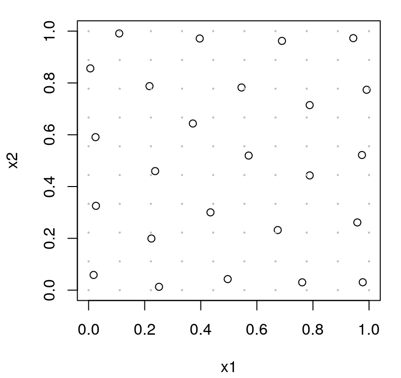
FIGURE 6.6: Approximate IMSPE design (6.5) by averaging over a reference set (gray dots). Compare to Figure 6.4.
This is a good approximation to Figure 6.4’s closed-form analog, but not perfect. You might say it’s missing a distinct feature of IMSPE-based design: avoiding boundaries. Design sites are not perfectly aligned with the boundary, but nearly so. Trouble is, design locations want to be close to reference set elements, and the reference set has almost as many points on the boundary as in the interior. A continuous analog, by contrast, would put measure zero on the boundary (a 1d manifold) relative to the full volume of the space (a 2d surface).
A different setting of the hyperparameters (say theta=0.5) reveals other inefficiencies due to discrete Xref. I encourage the curious reader to try this offline. Such drawbacks are an artifact of proposed random swaps having two hurdles to overcome in order to be accepted: 1) be farther from the previous “closest”; 2) but still just as close to a reference location. In the limit of a fully dense reference grid, i.e., an integral over an uncountable space, this second hurdle is always surmounted. Search based on our approximate criteria is more discrete than its closed form cousin, or even than maxent, and thus more difficult to solve. (Discrete and mixed continuous-discrete optimizations are harder than purely continuous ones.) A denser grid offers a partial solution, making the approximate criteria more accurate (at greater computational expense) but the nature of search is no less discrete.
Pivot now to the positive and consider how the approximate method can be applied in greater generality. What if we make the reference set occupy a smaller non-regular space? For example, as a somewhat contrived but certainly illustrative scenario, suppose we’re interested in predicting within intersecting ellipsoids centered on \((x_1,x_2) = (0.25, 0.25)\). Code below utilizes a random reference grid from two bivariate Gaussians meeting that description, effectively up-weighting locations closer to \((0.25, 0.25)\); an implicit \(w(\cdot)\).
Xref <- rmvnorm(100, mean=c(0.25, 0.25),
  sigma=0.005*rbind(c(2, 0.35), c(0.35, 0.1)))
Xref <- rbind(Xref,
  rmvnorm(100, mean=c(0.25, 0.25),
    sigma=0.005*rbind(c(0.1, -0.35), c(-0.35, 2))))
X <- imspe(25, 2, Xref=Xref)
Figure 6.7 shows the chosen design and reference set.
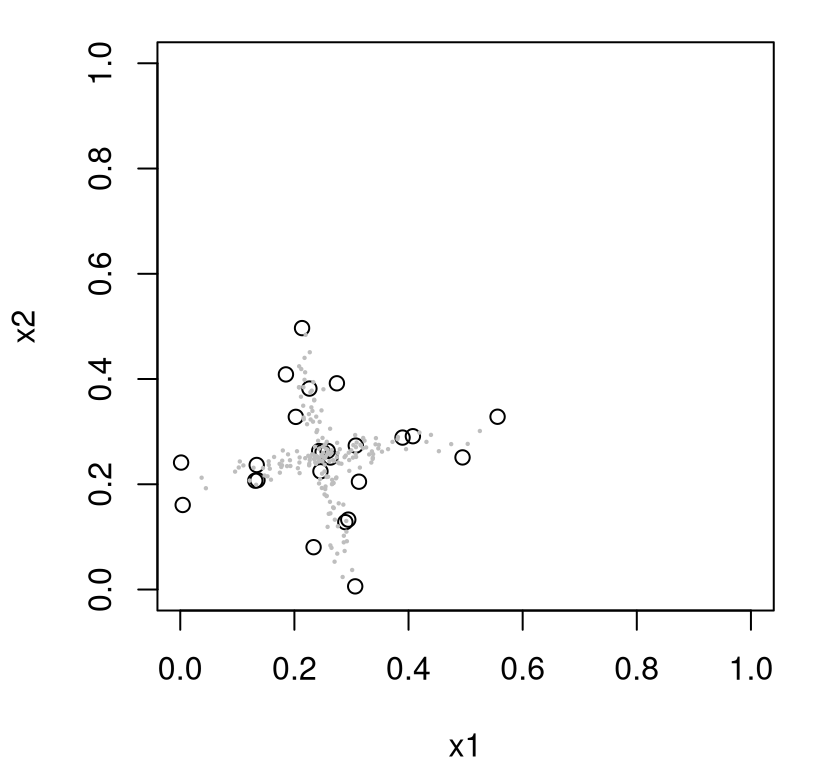
FIGURE 6.7: Approximate IMSPE design (6.5) with a reference set concentrated on a target study area.
Observe how the criteria organically attracts design locations to the reference set, but otherwise encourages some spread among selected sites. Spacing isn’t perfect, but that can be attributed to the nature of the approximate criteria, and to imperfect stochastic search. Both are improved with a larger reference set and more stochastic exchange proposals, at the expense of further computation. More efficient variations stem from a sequential design adaptation, presented shortly, and from a derivative-based search, which will have to wait until §9.3.5. Notice that some sites are chosen outside of the outermost Xref locations. It’s tempting to attribute this to approximation inefficiency, but in fact that phenomena is a direct consequence of the underlying IMSPE criterion. IMSPE resolves a tension between spreading out sites relative to one another, yet having them close to \(\mathcal{X}\). Recall that we have a stationary model, meaning that spread (on multiple scales) in the design is a prime player, even if we’re only interested in predicting locally, say in a sub-region of the input space. A more detailed discussion is left to §9.3.
6.2 Sequential design/active learning
A greedy, sequential approach to design is not just easier, it can also be more practical than the one-shot approach presented above. In many situations, selecting one design point at a time works better than static, single-batch design. For the technical junkie there are connections to non-sequential analogs, framed as approximations, but to settings where “true” hyperparameterization is known. Truth is in quotes since that’s never known in practice.
Sequential selection is also more computationally reasonable, being both better behaved numerically and also faster. That’s not to say that sequential methods always use fewer flops than batch selection. Often they do not. Yet extra computation versus alternatives (e.g., additional matrix decompositions), in situations where it’s warranted, have redeemed value in terms of the guidance that appropriately estimated quantities, tempered over many iterations of design acquisition, provide to searches that target both modeling and design goals. It’s easy to forget that design and modeling go hand-in-hand. Design impacts inference and calculations thereupon impact design, and all too often that’s not acknowledged when formally describing design goals. In case it’s not obvious, I’m uncomfortable with the idea of committing to a design before collecting (a modest amount of) data.
Figure 6.8 summarizes a sequential design setup. Although there are variations, here I shall emphasize the simple setup of augmenting an initial design by one, repeated until a desired size is reached.
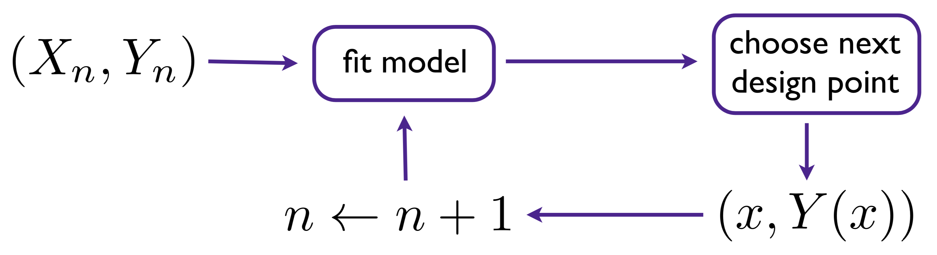
FIGURE 6.8: Diagram of sequential design/active learning/design augmentation.
To supplement that cartoon, consider Algorithm 6.1. The development here is a little backwards, saying what the algorithm is before delving into its key components, in particular Step 3 where a criterion is optimized to choose the next design element. Figure 6.8 is suggestive of indefinite updating, augmenting a design by one in each pass through the circuit. Algorithm 6.1 assumes a fixed total design size \(N\), iterating in \(n = n_0, \dots, N\), starting from a small seed design of size \(n_0\).
Algorithm 6.1: Sequential Design/Active Learning
Assume a flexible surrogate, e.g., a GP model, but with potentially unknown hyperparameterization.
Require a function \(f(\cdot)\) providing outputs \(y\sim f(x)\) for inputs \(x\), either deterministic or observed with noise; a choice of initial design size \(n_0\) and final size \(N\); and criterion \(J(x)\) to search for design augmentation.
Then
- Run a small seed, or bootstrapping experiment.
- Create an initial seed design \(X_{n_0}\) with \(n_0\) runs. Typically \(X_{n_0}\) is a model-free choice, e.g., derived from a static LHS or maximin design.
- Evaluate \(y_i \sim f(x_i)\) under each \(x_i^\top\) in the \(i^{\mathrm{th}}\) row of \(X_{n_0}\), for \(i=1,\dots, n_0\), obtaining \(D_{n_0} = (X_{n_0}, Y_{n_0})\).
- Set \(n \leftarrow n_0\), indexing iterations of sequential design.
- Fit the surrogate (and hyperparameters) using \(D_n\), e.g., via MLE.
- Solve criterion \(J(x)\) based on the fitted model from Step 2, resulting in a choice of \(x_{n+1} \mid D_n\) via \(x_{n+1} = \mathrm{argmax}_{x \in \mathcal{X}} \; J(x) \mid D_n.\)
- Observe the response at the chosen location by running a new simulation, \(y_{n+1} \sim f(x_{n+1})\).
- Update \(D_{n+1} = D_n \cup (x_{n+1}, y_{n+1})\); set \(n \leftarrow n+1\) and repeat from Step 2 unless \(n = N\).
Return the chosen design and function evaluations \(D_N\), along with surrogate fit (i.e., after a final application of Step 2).
Some commentary is in order. Consider Step 2. Numerical optimization of the likelihood to infer hyperparameters can require initial values. Random initialization is common when \(n\) is small, e.g., \(n = n_0\). Initializing with hyperparameters found in earlier iterations of sequential design – a warm start – offers computationally favorable results (faster convergence) and negligible deleterious effects when \(n\) is large. Earlier on, periodic random reinitialization can confer a certain robustness in the face of multimodal likelihoods (§5.3.4), which are not an uncommon occurrence. Skipping expensive \(\mathcal{O}(n^3)\) calculations in Step 2, e.g., using MLE calculations from earlier \(n\), is risky but could represent a huge computational savings: taking flops in \(\mathcal{O}(n^3)\) down to \(\mathcal{O}(n^2)\) using the updating equations in §6.3.
Step 3 in the algorithm presumes maximization, but it may be that minimization is more appropriate for the chosen criterion. Many flavors of optimization can be employed here. For example: evaluating \(J(x)\) on a candidate set of inputs \(\mathcal{X}\) in a discrete and/or randomized search; numerical optimization with optim in the case of compact \(\mathcal{X}\), potentially with help from closed-form derivatives. Warm-starting with \(x_n\) from previous iterations could be advantageous depending on the criterion, especially under variations considered for optimization in Chapter 7. When targeting global predictive accuracy or maximum information through learning, a more diverse (even random) initialization may be preferred in order to cope with highly multimodal objective surfaces. Note that \(J(x)\) evaluations can require forms for the predictive distribution \(Y(\mathcal{X}) \mid D_n\), e.g., kriging equations (5.3) in the GP case, or other aspects of fit conditional on hyperparameters from Step 2, and/or derivatives thereof.
In what follows, I introduce several criteria paired with an implementation of Steps 2–3 of Algorithm 6.1. Each is positioned as a pragmatic compromise between myriad alternatives. For example, I always warm start MLE calculations, but optimize criteria with optim under both random and warm-started initialization. Derivatives are used for the former but not the latter. Criteria are often easy to differentiate, and pointers are provided for the curious reader, however these are not implemented by our preferred library (laGP) under all variations considered below. §9.3.5 and Chapter 10 furnish derivatives accompanied by library routines for two important IMSPE-based sequential criteria in a slightly more ambitious setting.
6.2.1 Whack-a-mole: active learning MacKay
The simplest sequential design scheme for GPs, but it’s of course more widely applicable, involves choosing the next point to maximize predictive variance. Given data \(D_n = (X_n, Y_n)\), infer unknown hyperparameters \((\tau^2, \theta, g)\) by maximizing the likelihood, say, and choose \(x_{n+1}\) as
\[ x_{n+1} = \mathrm{argmax}_{x \in \mathcal{X}} \; \sigma_n^2(x). \]
Obtain \(y_{n+1} = Y(x_{n+1}) = f(x_{n+1}) + \varepsilon\); combine to form the new dataset: \(D_{n+1} = ([X_n; x_{n+1}^\top], [Y_n; y_{n+1}])\); repeat. In other words, the criterion provided to Algorithm 6.1 is \(J(x) \mid D_n \equiv \sigma_n^2(x)\), where \(\sigma_n^2(x)\) comes from kriging equations (5.3) applied using \((\hat{\tau}_n^2, \hat{\theta}_n^2, \hat{g}_n)\) trained on data compiled from earlier sequential design iterations: \(D_n = (X_n, Y_n)\). The \(n\) in the subscript is included to remind readers that the estimator is trained on data \(D_n\).
Simple right? But does it work well? In many cases, yes. MacKay (1992) argues that, in a certain sense, repeated application of such selection approximates a maximum entropy design. MacKay was working with neural networks. Almost a decade later, Seo et al. (2000) ported the idea to GPs, dubbing the method Active learning MacKay (ALM). After deriving GP updating equations in §6.3 we’ll be able to make a direct link between \(\sigma_n^2(x_{n+1})\) and \(|K_{n+1}|\), establishing for GPs the connection MacKay made for neural networks.
Active learning is ML jargon for sequential design. Online data selection is sometimes viewed as an example of reinforcement learning, which is itself a special case of optimal control. Criteria for sequential data selection, and their solvers, are known as acquisition functions in the active learning literature. In many ways, machine learners have been more “active” in sequential design research of late than statisticians have, so many have adopted their nomenclature. Active learning is where the learning algorithm gets to actively acquire the examples it’s trained on, creating a virtuous cycle between information acquisition and inference.
To demonstrate ALM, let’s revisit our favorite 2d dataset from §5.1.2, seeding with a small LHS of size \(n_0 = 12\). The code chunk below implements Step 1 of Algorithm 6.1 with this choice of \(f(\cdot)\).
library(lhs)
ninit <- 12
X <- randomLHS(ninit, 2)
f <- function(X, sd=0.01)
 {
  X[,1] <- (X[,1] - 0.5)*6 + 1
  X[,2] <- (X[,2] - 0.5)*6 + 1
  y <- X[,1] * exp(-X[,1]^2 - X[,2]^2) + rnorm(nrow(X), sd=sd)
 }
y <- f(X)
Step 2 involves fitting a model. Below, an isotropic GP is fit using laGP library routines.
library(laGP)
g <- garg(list(mle=TRUE, max=1), y)
d <- darg(list(mle=TRUE, max=0.25), X)
gpi <- newGP(X, y, d=d$start, g=g$start, dK=TRUE)
mle <- jmleGP(gpi, c(d$min, d$max), c(g$min, g$max), d$ab, g$ab)
Lest you spot it on your own and think it’s a sleight-of-hand, notice how darg specifies a maximum lengthscale of \(\theta_{\max} = 0.25\), a stark departure from earlier examples with these data. This kludge for d$max is crucial to obtaining consistently good results in repeated Rmarkdown builds. Pathological random \(n_0 = 12\)-sized seed LHS designs X, and associated noisy y-values, sometimes lead to GP fits that characterize a high-noise/low-signal regime via long lengthscales \(\hat{\theta}_{n_0}\) in an unconstrained setting. As a consequence, the predictive variance \(\sigma^2(\cdot)\) is highest at the edges of the design space, leading to \(x_{n+1}\)-values being selected there. Since the true \(f(\cdot)\) is nearly zero at all points on the boundary, that acquisition perpetuates a high-noise regime, creating a feedback loop where sites are never (or almost never) selected in the interior. The curious reader may wish to re-run the entirety of the code in this section with max=0.25 deleted to see what can happen. (It might take a few tries to get a bad result.)
Specifying preference for a relatively low \(\hat{\theta}_{n_0}\), effectively providing a strong prior on small lengthscale values and entirely precluding large ones, serves as a workaround. Using a larger \(n_0\) also helps, but would have diminished the value of our illustration. Better workarounds include a more thoughtful initial design, e.g., targeting a diversity of pairwise distances for more reliable \(\hat{\theta}_{n_0}\) (B. Zhang, Cole, and Gramacy 2020), and/or a more aggregate criteria like ALC (§6.2.2). But let’s table that for now, and continue with the illustration.
Before embarking on iterations of sequential design, it’ll help to establish some predictive quantities for later comparisons. R code below creates a testing grid and saves true (noiseless) responses at those locations.
For example, we may use these to calculate RMSE …
… in order to benchmark out-of-sample progress over iterations of design acquisition, \(n\), against commensurately-sized designs derived from similar criteria.
Predictive variance \(\sigma_n^2(x)\) produces football/sausage-shaped error-bars, so it must have many local maxima. In fact, it’s easy to see how the number of local maxima could grow linearly in \(n\). Optimizing globally over that surface presents challenges. Global optimization is a hard sequential design problem in its own right, hence Chapter 7. Here we shall stick to our favorite library-based local solver, optim with method="L-BFGS-B" (Byrd et al. 1995). Code below establishes the ALM objective as minus predictive variance, with the intention of passing to optim whose default is to search for minima.
Our success on a more global front will depend upon how clever we can be about initializing local solvers in a multi-start scheme. Suppose we “design” a collection of starting locations placed in parts of the input space known to have high variance, i.e., at the widest part of the sausage – as far as possible from existing design locations. This is basically what our sequential mymaximin function (§4.2.1) was created to do, encouraging spread in new (ALM search starting) locations relative to one another and to existing locations (\(X_n\) from previous iterations). Rather than paste mymaximin in here, it’s loaded in the Rmarkdown source behind the scenes. Alternatively, any of the variations entertained in response to §4.4 homework exercises may be preferred for more computationally efficient initialization.
Since there are about as many modes in \(\sigma_n^2(x)\) as inputs \(X_n\), it seems sensible to default to \(n\) space-filling multi-start locations for ALM searches. The function below facilitates search for \(x_{n+1}\), coded as xnp1, implementing of Step 3 of Algorithm 6.1. It’s designed to be somewhat generic to searching objective (obj), which we provide as obj.alm by default but anticipate variations on the horizon. Execution begins by creating a sequential maximin design of multi-start initializers. It then iterates over optim calls with obj. Notice that this implementation is tailored to 2d inputs, as is everything supporting the rest of this example. However it wouldn’t be hard to make things more generic with small edits in a few places.
xnp1.search <- function(X, gpi, obj=obj.alm, ...)
 {
  start <- mymaximin(nrow(X), 2, T=100*nrow(X), Xorig=X)
  xnew <- matrix(NA, nrow=nrow(start), ncol=ncol(X) + 1)
  for(i in 1:nrow(start)) {
    out <- optim(start[i,], obj, method="L-BFGS-B", lower=0,
      upper=1, gpi=gpi, ...)
    xnew[i,] <- c(out$par, -out$value)
  }
  solns <- data.frame(cbind(start, xnew))
  names(solns) <- c("s1", "s2", "x1", "x2", "val")
  return(solns)
 }
On output, a data.frame is returned combining starting and ending locations with a final column recording the value of the objective found by optim. Such comprehensive output is probably overkill for most situations, because all that matters is c(x1, x2) coordinates in the row having the smallest val. Other rows are furnished primarily to aid in illustration. For example, Figure 6.9 draws arrows connecting starting c(s1, s2) coordinates to locally optimal variance-maximizing solutions, with a red dot at the terminus of the best val arrow. (Any arrows with near-zero length are omitted, and occasionally such an arrow “terminates” at the red dot.)
solns <- xnp1.search(X, gpi)
plot(X, xlab="x1", ylab="x2", xlim=c(0,1), ylim=c(0,1))
arrows(solns$s1, solns$s2, solns$x1, solns$x2, length=0.1)
m <- which.max(solns$val)
prog <- solns$val[m]
points(solns$x1[m], solns$x2[m], col=2, pch=20)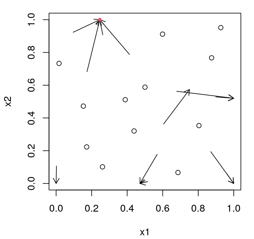
FIGURE 6.9: First iteration of ALM search. Each arrow represents an origin and outcome (terminus) of multi-start exploration of predictive variance. Variance-maximizing location is indicated as a red dot.
Considering the random nature of this Rmarkdown example, it’s hard to speculate on details in Figure 6.9. Often several arrows terminate at the same location. At this early stage of sequential design the most likely location for the red dot, and indeed the terminus of many arrows, is somewhere along the boundary of the input space.
Step 4 in Algorithm 6.1 involves running \(y \sim f(x_{n+1})\) at the new input location – the red dot. Then add the new pair into the design in Step 5.
Implementing an intermediate calculation, spanning Step 5 of the current iteration and Step 2 of the next, the updateGP function below augments an existing GP object, referenced here by gpi, with new input–output pairs. This is a very fast update, leveraging \(\mathcal{O}(n^2)\) calculations detailed in §6.3. However, the penultimate line in the code chunk below updates MLE calculations on hyperparameters at \(\mathcal{O}(n^3)\) expense, completing a loop back up to Step 2 of Algorithm 6.1. Often convergence is achieved after very few likelihood evaluations when carrying on from where search terminated in the previous sequential design iteration, i.e., at the MLE setting under just one fewer training data points. The final line below records an RMSE value (under the new design) on the hold-out testing set (which is the same as before). This step is not formally part of Algorithm 6.1.
updateGP(gpi, xnew, y[length(y)])
mle <- rbind(mle, jmleGP(gpi, c(d$min, d$max), c(g$min, g$max),
d$ab, g$ab))
rmse <- c(rmse, sqrt(mean((yytrue - predGP(gpi, XX, lite=TRUE)$mean)^2)))Updated fit in hand, we’re ready for another active learning acquisition. The code below represents a second full pass through the loop in Algorithm 6.1, comprising the sequence of Steps \(3 \rightarrow 4 \rightarrow 5 \rightarrow 2\), ending with new MLE and RMSE calculations on the augmented design.
solns <- xnp1.search(X, gpi)
m <- which.max(solns$val)
prog <- c(prog, solns$val[m])
xnew <- as.matrix(solns[m, 3:4])
X <- rbind(X, xnew)
y <- c(y, f(xnew))
updateGP(gpi, xnew, y[length(y)])
mle <- rbind(mle, jmleGP(gpi, c(d$min, d$max), c(g$min, g$max),
d$ab, g$ab))
p <- predGP(gpi, XX, lite=TRUE)
rmse <- c(rmse, sqrt(mean((yytrue - p$mean)^2)))The outcome of that search is summarized by Figure 6.10, again with arrows and a red dot. Notice that the red dot from the previous iteration has been promoted to an open circle, now fully incorporated into the design.
plot(X, xlab="x1", ylab="x2", xlim=c(0,1), ylim=c(0,1))
arrows(solns$s1, solns$s2, solns$x1, solns$x2, length=0.1)
m <- which.max(solns$val)
points(solns$x1[m], solns$x2[m], col=2, pch=20)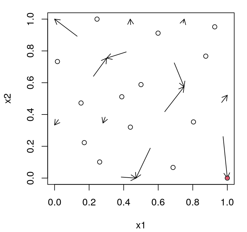
FIGURE 6.10: Second iteration of ALM search after Figure 6.9.
Again, it’s hard to speculate about the outcome of this search for the largest variance input location. Usually the result is intuitive considering locations of existing design points (open circles), and the origin and terminus of the arrows. Before turning to a more in-depth investigation into merits of this scheme, let’s do several more iterations through the loop, for a total of \(N=25\) runs. Again, this is Steps \(3 \rightarrow 4 \rightarrow 5 \rightarrow 2\) wrapped in a for loop.
for(i in nrow(X):24) {
solns <- xnp1.search(X, gpi)
m <- which.max(solns$val)
prog <- c(prog, solns$val[m])
xnew <- as.matrix(solns[m, 3:4])
X <- rbind(X, xnew)
y <- c(y, f(xnew))
updateGP(gpi, xnew, y[length(y)])
mle <- rbind(mle, jmleGP(gpi, c(d$min, d$max), c(g$min, g$max),
  d$ab, g$ab))
p <- predGP(gpi, XX, lite=TRUE)
rmse <- c(rmse, sqrt(mean((yytrue - p$mean)^2)))
}The mle object, shown in part below (every other iteration to save space), summarizes steps of our search vis-a-vis estimated lengthscale and nugget hyperparameters.
##          d        g tot.its dits gits
## 1  0.04110 0.002881      21    7   14
## 3  0.03679 0.002884       6    4    2
## 5  0.03499 0.002886       6    4    2
## 7  0.03544 0.002886       6    4    2
## 9  0.03568 0.002886       7    4    3
## 11 0.02890 0.002891       8    5    3
## 13 0.02742 0.002891       7    4    3
Bigger movements and more MLE iterations, especially for \(\theta\) (d and dits), are usually associated with earlier sequential design steps. More often than not, in repeated Rmarkdown builds, later searches are associated with smaller relative MLE moves, converging rapidly in just a few iterations, benefiting from warm starts provided by values stored in the GP object gpi from previous iterations. Perhaps full MLE updates, with jmlegp above, may not be required for subsequent sequential design iterations. That could represent substantial computational savings as \(n\) gets big, making updates take flops in \(\mathcal{O}(n^2)\) rather than \(\mathcal{O}(n^3)\).
Figure 6.11 summarizes the predictive surface after \(N=25\) design sites have been selected in this way. A mean surface is shown on the left, and standard deviation on the right. Numbers plotted indicate the iteration in which each site was chosen. Recall that the first \(n_0 = 12\) came from an LHS.
par(mfrow=c(1,2))
cols <- heat.colors(128)
image(x1, x2, matrix(p$mean, ncol=length(x1)), col=cols, main="mean")
text(X, labels=1:nrow(X), cex=0.75)
image(x1, x2, matrix(sqrt(p$s2), ncol=length(x1)), col=cols, main="sd")
text(X, labels=1:nrow(X), cex=0.75)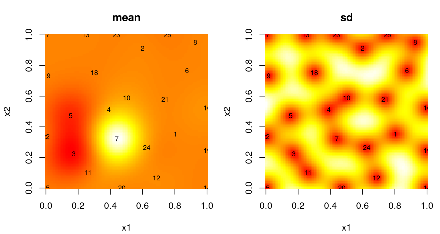
FIGURE 6.11: Predictive mean (left) and standard deviation (right) after ALM-based sequential design.
Those surfaces look reasonable, at least from a purely aesthetic perspective. A fair criticism is that the chosen sites are no better, or could perhaps be even worse, than what would have been obtained with a simple \(N=25\) space-filling design, i.e., calculated in a single batch at the outset. One nice feature, or byproduct, of a sequential model-based alternative is a measure of progress, namely the maximal variance used as the basis of each sequential design decision. We’ve been saving that as prog in the code above, so that these may be plotted like in Figure 6.12. Note that prog saves predGP(...)$s2, involving a \(\hat{\tau}^2_n\) estimate that changes from one acquisition to the next, \(n \rightarrow n+1\). Within a particular iteration this scale estimate has no impact on selection criteria, but between iterations it can cause prog to “jump”, up or down, depending on incoming \(y_{n+1}\)-values and corresponding hyperparameter updates. At this time, laGP doesn’t provide direct access to \(\hat{\tau}^2\) in order to correct this, if so desired.

FIGURE 6.12: ALM-progress over sequential design iterations.
Whether jumps are present in the figure or not – it depends on the random Rmarkdown build – it’s clear that progress has not yet leveled off. Consider 75 more iterations of active learning, stopping at \(N=100\). The code below duplicates the for loop above after reinitializing \(\hat{\theta} \equiv\) d, and removing the restrictive \(\hat{\theta}_{\max}=0.25\) setting. After \(n=25\) samples are chosen, an aggressive prior is not as important in order to avoid pathological behavior. (A conservative Bayesian approach has greatest value to the practitioner when data are few.)
d <- darg(list(mle=TRUE), X)
for(i in nrow(X):99) {
  solns <- xnp1.search(X, gpi)
  m <- which.max(solns$val)
  prog <- c(prog, solns$val[m])
  xnew <- as.matrix(solns[m, 3:4])
  X <- rbind(X, xnew)
  y <- c(y, f(xnew))
  updateGP(gpi, xnew, y[length(y)])
  mle <- rbind(mle, jmleGP(gpi, c(d$min, d$max), c(g$min, g$max),
    d$ab, g$ab))
  p <- predGP(gpi, XX, lite=TRUE)
  rmse <- c(rmse, sqrt(mean((yytrue - p$mean)^2)))
}
An inspection of MLEs found during each iteration reveals small changes in \(\hat{\theta}_n\) and \(\hat{g}_n\) on both relative and absolute terms. The number of iterations required for convergence can vary somewhat more substantially over longer search horizons, but is usually small.
##          d        g tot.its dits gits
## 14 0.02812 0.002890       7    4    3
## 24 0.03220 0.002864       7    3    4
## 34 0.02649 0.002853       8    4    4
## 44 0.03229 0.002555      10    6    4
## 54 0.03400 0.002083       8    4    4
## 64 0.03435 0.001915      13    6    7
## 74 0.03243 0.004924      44   21   23
## 84 0.03438 0.007699      23   11   12
As shown in Figure 6.13, progress metrics are starting to level off. The magnitude and frequency of jumps in prog, shown on the left, generally decreases over acquisition iterations. (If there were no jumps before, there are almost certainly some in this view.) Accuracy, measured by RMSE in the right panel, shows similar behavior, having leveled off substantially in the latter thirty-five iterations or so. Although an out-of-sample testing set is seldom available for use in this context, it’s nice to see a substantial degree of correlation between predictive accuracy and (maximal) predictive uncertainty, which is what was used to guide design.
par(mfrow=c(1,2))
plot((ninit+1):nrow(X), prog, xlab="n: design size", ylab="ALM progress")
plot(ninit:nrow(X), rmse, xlab="n: design size", ylab="OOS RMSE")
FIGURE 6.13: Maximum variance (left, lower is better) and out-of-sample RMSE (right) over 100 ALM acquisitions.
Figure 6.14 shows the posterior surface and the location of the chosen design sites.
par(mfrow=c(1,2))
image(x1, x2, matrix(p$mean, ncol=length(x1)), col=cols, main="mean")
text(X, labels=1:nrow(X), cex=0.75)
image(x1, x2, matrix(sqrt(p$s2), ncol=length(x1)), col=cols, main="sd")
text(X, labels=1:nrow(X), cex=0.75)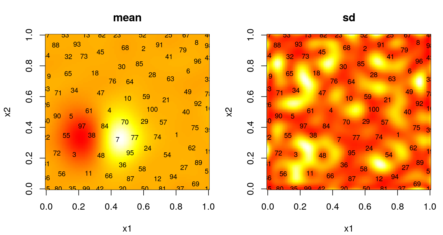
FIGURE 6.14: Predictive mean (left) and standard deviation (right) after ALM-based sequential design.
Observe dense coverage along the boundary, a telltale sign of maxent design. The degree of space-fillingness could be improved, but by proceeding sequentially less faith is required in the quality of an initial hyperparameterization. It can be instructive to repeat selection of these 100 design sites to explore variability in outcomes. ALM can misbehave, especially if the starting design is unlucky to miss strong signal in the data. When that happens, initial fits of hyperparameters favor noise, even when restricted by \(\hat{\theta}_{\max} = 0.25\), sparking a feedback loop from which the sequential procedure may fail to recover.
A more graceful solution, besides simply initializing with a larger design, could involve a more aggregate criteria. Maximizing variance is myopic. ALM doesn’t recognize that acquisitions impact predictive equations globally. Instead it “wacks down” the highest variance locations, a set of measure zero, potentially ignoring a continuum of fatter regions where uncertainty may cumulatively be much larger. This is why we end up with lots of sites on the boundary. Variance is high there because there are fewer data points nearby – there are none beyond the boundary, a situation which could not be remedied by any sequential data acquisition scheme. Yet those boundary locations are perhaps least useful when it comes to predicting elsewhere, being as far as possible from almost any notion of elsewhere.
6.2.2 A more aggregate criteria: active learning Cohn
You could say that ALM has somewhat of a scale problem. Just because predictive variance is high doesn’t mean that there’s value in adding more data. (I’m thinking ahead a little bit to Chapters 9–10 where noise variances may not be uniform in the input space.) One could instead work with epistemic variance (5.16), i.e., the variance of the latent field (§5.3.2), or variance of the mean. Operationally speaking, this amounts to using a zero nugget when calculating out-of-sample covariances among \(\mathcal{X} \equiv\) XX. But that only helps to a degree. High variance may well be an accurate inference for the problem at hand, which would mean seriously diminishing returns to further data acquisition. A better metric might be reduction in variance. That is, how helpful is a potential new design site at reducing predictive uncertainty? If a lot, relative to previous reductions and relative to other new design sites, then it could be quite helpful to perform a new run at that location. If not, perhaps another location would be preferred or perhaps we have enough data already.
But this begs the question where; where should the reduction be measured? One option is everywhere, integrating over the entire input space like IMSPE does for global design (§6.1.2). Such an integral is tractable analytically for rectangular input spaces, but I shall defer that discussion to Chapter 10. At the other extreme is measuring reduction in variance at a particular reference location, or at a collection of locations, thereby approximating the integral with a sum like we did with IMSPE (6.5). The first person to suggest such an acquisition heuristic in a nonparametric regression context was Cohn (1994), for neural networks. As with ALM, Seo et al. (2000) adapted Cohn’s idea to GPs and called it active learning Cohn (ALC). The result is essentially a sequential analog of IMSPE design, and in fact the sequential version can be shown to approximate a full \(A\)-optimal design.
How does it all work? Recall that predictive variance follows
\[ \sigma_n^2(x) = \hat{\tau}_n^2[1 + \hat{g}_n - k^\top_n(x) K_n^{-1} k_n(x) ] \quad \mbox{ where } \quad k_n(x) \equiv C_{\hat{\theta}_n}(X_n, x), \]
written here with an \(n\) subscript on all estimated quantities in order to emphasize their dependence on data \(D_n = (X_n, Y_n)\) via \(\hat{\tau}_n^2\), \(\hat{g}_n\), and \(\hat{\theta}_n\) hidden inside \(K_n\). Let \(\tilde{\sigma}_{n+1}^2(x)\) denote the deduced variance based on design \(X_{n+1}\) combining \(X_n\) and a new input location \(x_{n+1}^\top\) residing in its \(n+1^{\mathrm{st}}\) row. Otherwise, \(\tilde{\sigma}_{n+1}^2(x)\) conditions on the same estimated quantities as \(\sigma_n^2(x)\), i.e., \(\hat{\tau}_n^2\), \(\hat{g}_n\), and \(\hat{\theta}_n\), all estimated from \(Y_n\). Since \(Y_n\) doesn’t directly appear in \(\sigma_n^2(x)\), nor would it directly appear in \(\tilde{\sigma}_{n+1}^2(x)\). Therefore, quite simply
\[\begin{equation} \tilde{\sigma}_{n+1}^2(x) = \hat{\tau}_n^2[1 + \hat{g}_n - k^\top_{n+1}(x) K_{n+1}^{-1} k_{n+1}(x) ] \quad \mbox{ where } \quad k_{n+1}(x) \equiv C_{\hat{\theta}_n}(X_{n+1}, x). \tag{6.6} \end{equation}\]
Using that definition, the ALC criteria is the average (integrated over \(\mathcal{X}\) or any other subset of the input space) reduction in variance from \(n \rightarrow n+1\) measured through a choice of \(x_{n+1}\), augmenting the design:
\[ \begin{aligned} \Delta \sigma_n^2(x_{n+1}) &= \int_{x \in \mathcal{X}} \sigma_n^2(x) - \tilde{\sigma}_{n+1}^2(x) \;dx\\ &= c - \int_{x \in \mathcal{X}} \tilde{\sigma}_{n+1}^2(x) \; dx. \end{aligned} \]
Wishing predictive uncertainty to be reduced as much as possible, that translates into finding an \(x_{n+1}\) maximizing \(\Delta \sigma_n^2(x_{n+1})\). But that’s the same as minimizing the integrated deduced variance. Therefore the criterion that must be solved in each iteration of sequential design, occupying Step 3 of Algorithm 6.1, is
\[\begin{equation} x_{n+1} = \mathrm{argmin}_{x \in \mathcal{X}} \int_{x \in \mathcal{X}} \tilde{\sigma}_{n+1}^2(x) \; dx. \tag{6.7} \end{equation}\]
A closed form for rectangular \(\mathcal{X}\), complete with derivatives for maximizing, is provided later in Chapter 10. Often in practice the integral is approximated by a sum over a reference set (6.5) as this offers the simplest, most general, implementation. Although a singleton reference set (\(\mathcal{X} = x_{\mathrm{ref}}\), dropping the integral or sum entirely) represents a degenerate case where \(x_{n+1} = x_{\mathrm{ref}}\), any larger reference set demands \(x_{n+1}\) make a trade-off that considers broader impact on variance reduction when new data are added into the design. The laGP package has functions called alcGP and alcGPsep that automate this objective, providing evaluations of \(\Delta \sigma_n^2(x_{n+1})\) to within additive and multiplicative constants. More specifically, the output is scale-free, having “divided out” \(\hat{\tau}_n^2\) in a manner similar to IMSPE (§6.1.2). Since we wish to maximize this quantity, the wrapper below negates the output of alcGP. It also uses the square root, which conveys a more numerically stable objective for optimization with optim. Since the square root is a monotone transformation, the location of stationary points is unchanged.
Our xnp1.search from §6.2.1, solving for the next input \(x_{n+1}\), was designed to be generic enough to accommodate other objective functions and arguments, like obj.alc and Xref, through ellipses (...). Before jumping into an illustration, we must clean up our ALM search and reinitialize a new GP with the same ninit starting values. This will help control variability for subsequent comparison between ALC and ALM-based sequential designs.
deleteGP(gpi)
X <- X[1:ninit,]
y <- y[1:ninit]
g <- garg(list(mle=TRUE, max=1), y)
d <- darg(list(mle=TRUE, max=0.25), X)
gpi <- newGP(X, y, d=d$start, g=g$start, dK=TRUE)
mle <- jmleGP(gpi, c(d$min, d$max), c(g$min, g$max), d$ab, g$ab)
p <- predGP(gpi, XX, lite=TRUE)
rmse.alc <- sqrt(mean((yytrue - p$mean)^2))
The code below invokes the first iteration of ALC search. A 100-element LHS is chosen for reference set Xref, but otherwise the process is similar to that for ALM except that obj.alc and Xref are provided to xnp1.search.
Xref <- randomLHS(100, 2)
solns <- xnp1.search(X, gpi, obj=obj.alc, Xref=Xref)
m <- which.max(solns$val)
xnew <- as.matrix(solns[m, 3:4])
prog.alc <- solns$val[m]
Figure 6.15 offers a visual summary of the search, with arrows and a red dot showing the chosen \(x_{n+1}\) location. Smaller filled-gray dots denote Xref.
plot(X, xlab="x1", ylab="x2", xlim=c(0,1), ylim=c(0,1))
arrows(solns$s1, solns$s2, solns$x1, solns$x2, length=0.1)
points(solns$x1[m], solns$x2[m], col=2, pch=20)
points(Xref, cex=0.25, pch=20, col="gray")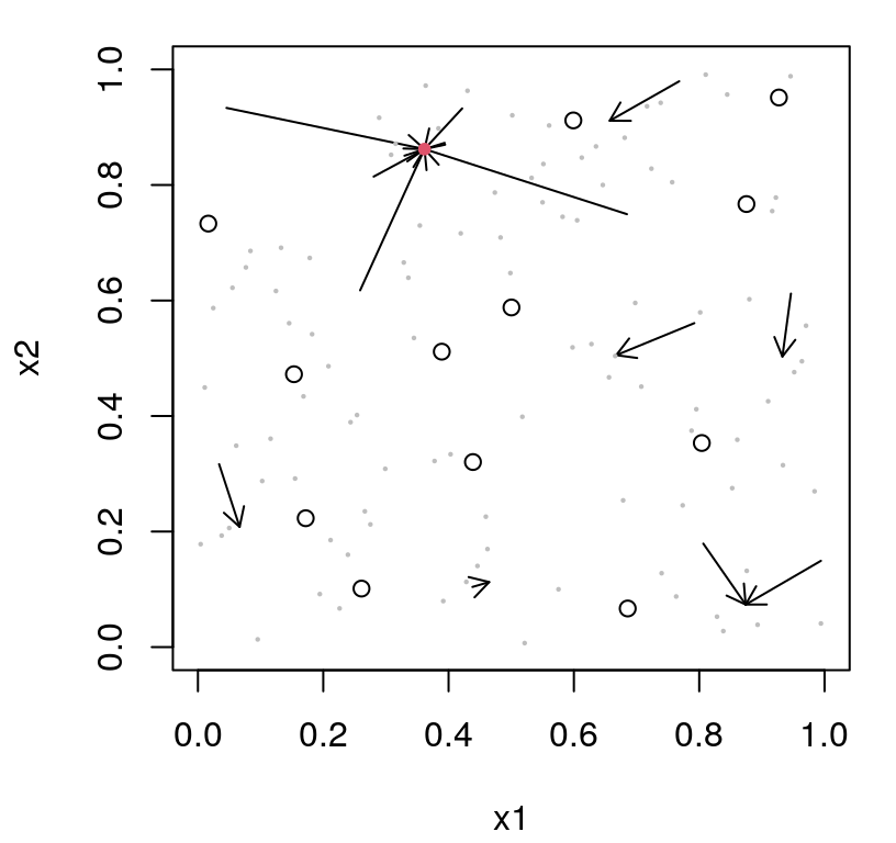
FIGURE 6.15: First iteration of ALC search in the style of Figure 6.9. Gray dots denote reference locations.
Domains of attraction from the ALC criterion are similar to ALM’s, however global optima are more likely to be in the interior for ALC. In part, this is because ALC prefers candidates which are far from \(X_n\) and close to Xref. Since Xref is an LHS, very few are found near the boundary. Although it’s hard to speculate on a location selected for a particular Rmarkdown build, especially considering the random nature of the reference set used by ALC, the chosen location for \(x_{n+1}\) in the version I’m looking at now is indeed in the interior. Code below gathers \(y(x_{n+1})\), and updates the GP predictor to get ready for the next acquisition by ALC.
X <- rbind(X, xnew)
y <- c(y, f(xnew))
updateGP(gpi, xnew, y[length(y)])
mle <- rbind(mle, jmleGP(gpi, c(d$min, d$max), c(g$min, g$max),
  d$ab, g$ab))
p <- predGP(gpi, XX, lite=TRUE)
rmse.alc <- c(rmse.alc, sqrt(mean((yytrue - p$mean)^2)))
Skipping ahead a bit, the loop below fills out the rest of the design in this way, up to \(N=100\). This for loop is identical to the ALM analog, except using ALC with obj.alc and Xref instead. Notice that Xref is refreshed for each acquisition. This helps encourage diversity in search from one iteration to the next. Although any single reference set may lead to a poor sum-based approximation of the integral behind ALC (6.7) in any particular acquisition iteration, a diversity of (even small) reference sets limits the influence of bad behavior on aggregate.
d <- darg(list(mle=TRUE), X)
for(i in nrow(X):99) {
  Xref <- randomLHS(100, 2)
  solns <- xnp1.search(X, gpi, obj=obj.alc, Xref=Xref)
  m <- which.max(solns$val)
  prog.alc <- c(prog.alc, solns$val[m])
  xnew <- as.matrix(solns[m, 3:4])
  X <- rbind(X, xnew)
  y <- c(y, f(xnew))
  updateGP(gpi, xnew, y[length(y)])
  mle <- rbind(mle, jmleGP(gpi, c(d$min, d$max), c(g$min, g$max),
    d$ab, g$ab))
  p <- predGP(gpi, XX, lite=TRUE)
  rmse.alc <- c(rmse.alc, sqrt(mean((yytrue - p$mean)^2)))
}
Updates to hyperparameter MLEs are saved above, however the values recorded look similar to those from ALM so they’re not shown here. Figure 6.16 provides a view into progress over iterations of ALC-based acquisition.
par(mfrow=c(1,2))
plot((ninit+1):nrow(X), prog.alc, xlab="n: design size",
  ylab="ALC progress")
plot(ninit:nrow(X), rmse, xlab="n: design size", ylab="OOS RMSE")
points(ninit:nrow(X), rmse.alc, col=2, pch=20)
legend("topright", c("alm", "alc"), pch=c(21,20), col=1:2)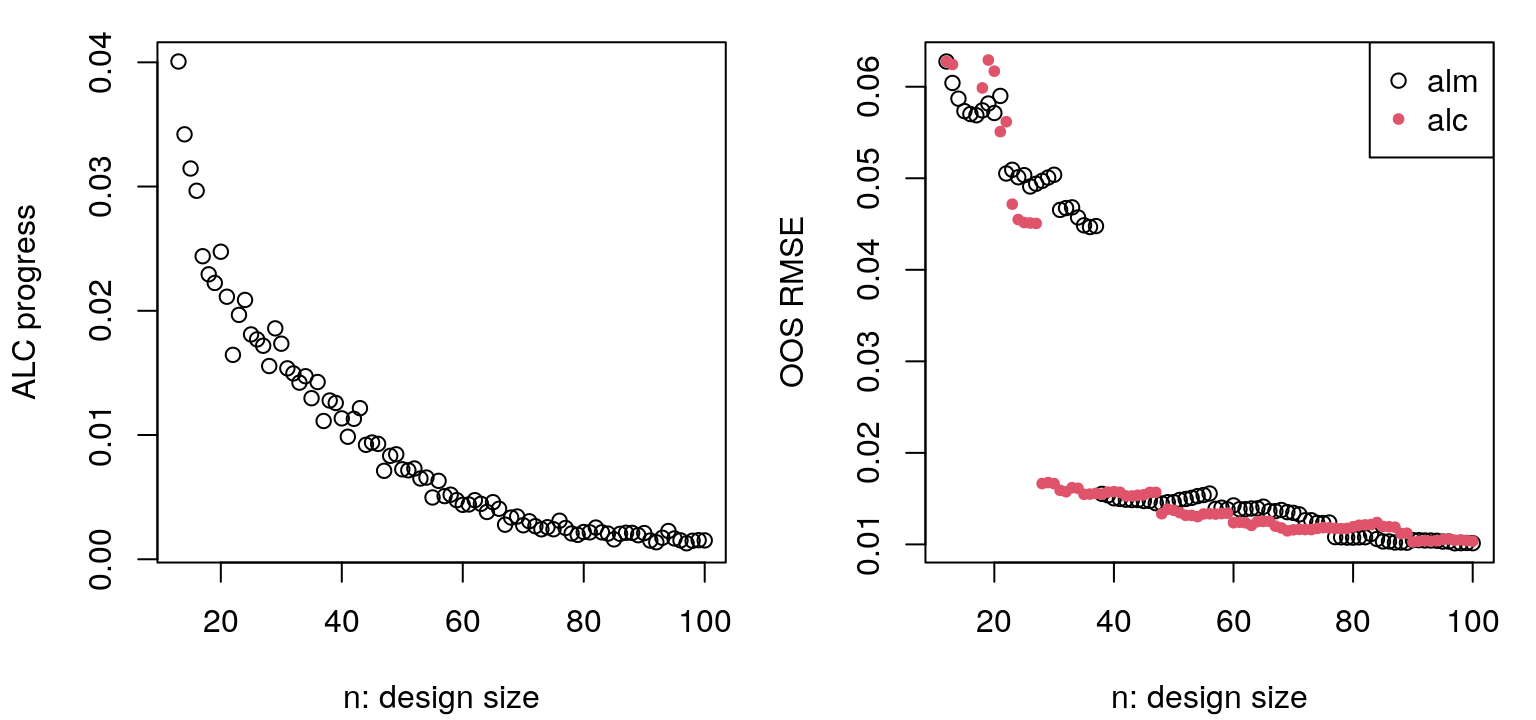
FIGURE 6.16: Progress in ALC sequential design in terms of integrated reduction in variance (left, lower is better) and out-of-sample RMSE (right), with comparison to ALM from Figure 6.12.
The left panel, showing progress on obj.alc, is less jumpy than the ALM analog, but also perhaps more noisy. It’s less jumpy because alcGP and alcGPsep factor out scale \(\hat{\tau}_n^2\). Noise arises due to novel random Xref in each iteration of design; a fixed Xref would smooth things out considerably, but bias search. Observe that progress on the ALC criteria is flattening out in later iterations. On the right is out-of-sample RMSE as compared to ALM. Notice how they end at about the same place, but ALC gets there faster. While ALM is busy filling out boundaries in early iterations, ALC is filling in interior regions which are closer to the vast majority of inputs in the testing set. Figure 6.17 shows predictive mean and standard deviation, with locations and order of selected design sites overlayed.
par(mfrow=c(1,2))
image(x1, x2, matrix(p$mean, ncol=length(x1)), col=cols, main="mean")
text(X, labels=1:nrow(X), cex=0.75)
image(x1, x2, matrix(sqrt(p$s2), ncol=length(x1)), col=cols, main="sd")
text(X, labels=1:nrow(X), cex=0.75)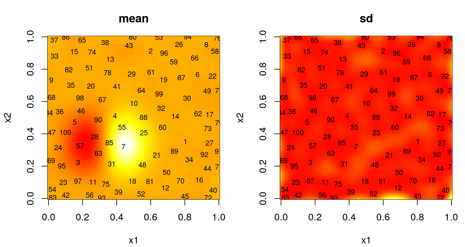
FIGURE 6.17: Predictive mean (left) and standard deviation (right) after ALC-based sequential design.
Coverage of the boundary is sparser, but perhaps not as sparse as what we saw from static IMSPE design in §6.1.2. Predictive uncertainty is higher for ALC than ALM along that boundary, but those regions are not favored by ALC as their remote location makes them poor for driving down variance at reference sites; i.e., they’re less than ideal for driving down uncertainty aggregated across the entirety of the input space.
6.2.3 Other sequential criteria
Several other heuristics have been proposed in the literature, some of which will be the subject of future chapters – particularly when the target is optimization. One that pops up often involves the Fisher information (FI) of kernel hyperparameters, particularly lengthscale(s) \(\theta\). The equations are a little cumbersome, involving second derivatives and expectations as FI calculations often do. Rather than duplicate these here, allow me to refer the interested reader to the appendix of Gramacy and Apley (2015). Search via FI is implemented by fishGP in the laGP package.
One attractive aspect of FI, compared to ALC say, is that no reference set is required. The criterion’s emphasis on learning parameters means that it’s less sensitive to initial choices for those parameters, but since FI is ultimately evaluated under \(\hat{\theta}_n\), from the previous iteration \(n\), there’s still some degree of sensitivity and so we still have to be careful about initial values. A disadvantage is that FI doesn’t directly emphasize predictive accuracy, rather hyperparameter estimation. It usually does not lead to designs with the most accurate predictors. To see why, feed obj.fish into xnp1.search to sequentially build up a design with \(N=100\) input–output pairs.
X <- X[1:ninit,]
y <- y[1:ninit]
d <- darg(list(mle=TRUE, max=0.25), X)
gpi <- newGP(X, y, d=0.1, g=0.1*var(y), dK=TRUE)
mle <- jmleGP(gpi, c(d$min, d$max), c(g$min, g$max), d$ab, g$ab)
rmse.fish <- sqrt(mean((yytrue - predGP(gpi, XX, lite=TRUE)$mean)^2))
prog.fish <- c()
for(i in nrow(X):99) {
  solns <- xnp1.search(X, gpi, obj=obj.fish)
  m <- which.max(solns$val)
  prog.fish <- c(prog.fish, solns$val[m])
  xnew <- as.matrix(solns[m, 3:4])
  X <- rbind(X, xnew)
  y <- c(y, f(xnew))
  updateGP(gpi, xnew, y[length(y)])
  mle <- rbind(mle, jmleGP(gpi, c(d$min, d$max), c(g$min, g$max),
    d$ab, g$ab))
  p <-predGP(gpi, XX, lite=TRUE)
  rmse.fish <- c(rmse.fish, sqrt(mean((yytrue - p$mean)^2)))
}
Figure 6.18 shows the design and the resulting fit, which illustrates striking differences compared to earlier analogs.
par(mfrow=c(1,2))
image(x1, x2, matrix(p$mean, ncol=length(x1)), col=cols, main="mean")
text(X, labels=1:nrow(X), cex=0.75)
image(x1, x2, matrix(sqrt(p$s2), ncol=length(x1)), col=cols, main="sd")
text(X, labels=1:nrow(X), cex=0.75)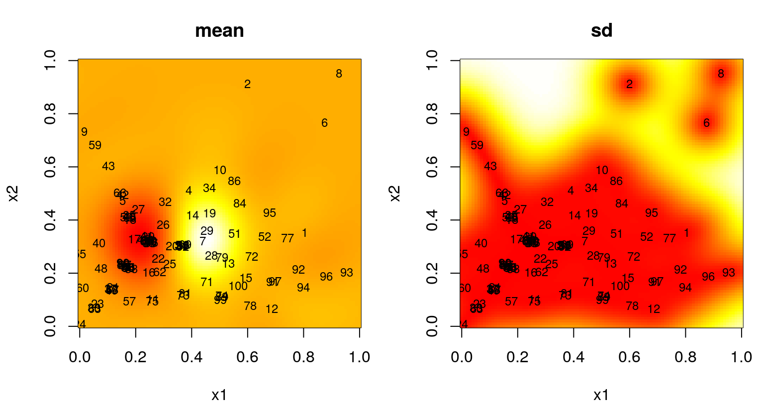
FIGURE 6.18: Predictive mean (left) and standard deviation (right) after an FI-based sequential design.
There’s a certain “clumpiness”, but also definitely a pattern in selected sites. Whole swaths of the input space are missing locations. This is the result of FI preferring distances between inputs on different scales, which makes sense in order to best learn lengthscale. Whether or not the densely sampled locations coincide with the “interesting part” of the response surface, in this case the “bumps” in the lower-left-hand quadrant, is largely a matter of luck. Repeated builds of this Rmarkdown document lead to dramatically different RMSE progress metrics over time, as shown for one instance in the right panel of Figure 6.19. This happens even though progress on the FI metric, as shown in the left panel, is remarkably consistent. If design acquisitions are lucky to cluster near the bumps, then the fact that the responses are conveniently zero elsewhere – and that our GP is zero-mean reverting – leads to excellent RMSEs compared to ALM and ALC. An unlucky clumping can lead to disastrous RMSE calculations.
par(mfrow=c(1,2))
plot((ninit+1):nrow(X), prog.fish, xlab="n: design size",
  ylab="FI progress")
plot(ninit:nrow(X), rmse, xlab="n: design size", ylab="OOS RMSE")
points(ninit:nrow(X), rmse.alc, col=2, pch=20)
points(ninit:nrow(X), rmse.fish, col=3, pch=19)
legend("topright", c("alm", "alc", "fish"), pch=21:19, col=1:3)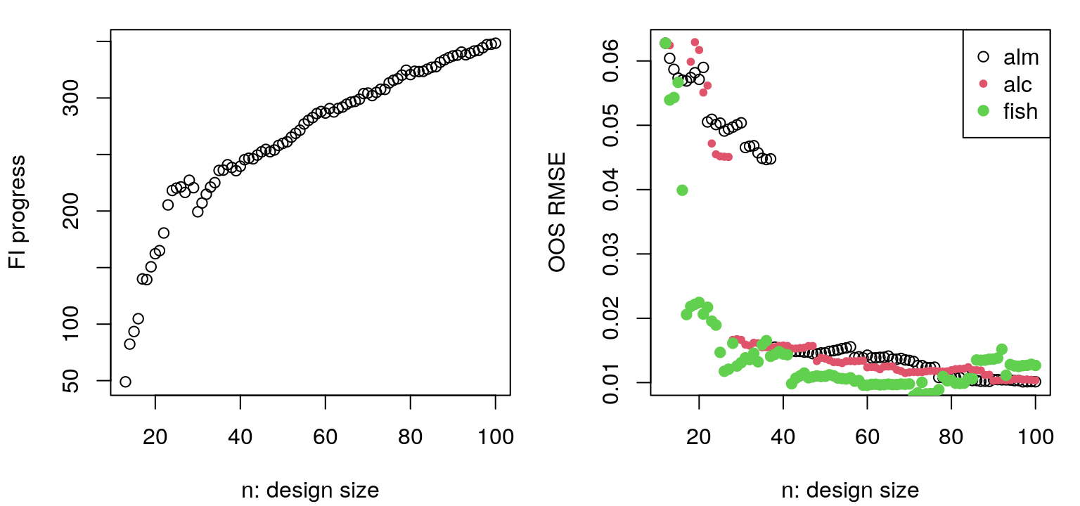
FIGURE 6.19: Progress in terms of FI (left, higher is better) and out-of-sample RMSE as compared to previous heuristics.
Readers are strongly encouraged to repeat the code above to explore that variability. If ALC and ALM are somewhat unsatisfying in that they basically produce space-filling designs with the burden of initializing GP hyperparameters for stable performance over the iterations, FI is unsatisfying in that design targeting good hyperparameters is insufficient for what’s usually the primary goal: prediction. A hybrid approach however, first FI to learn parameters then ALC for accurate prediction, may represent an advantageous compromise. Still, FI needs an initial \(\hat{\theta}_{n_0}\) from somewhere.
Regarding \(\hat{\theta}_n\), sequential design acquisitions above are grossly inefficient from a computational perspective. MLE optimizations in \(\mathcal{O}(n^3)\) are carried out in each iteration, from \(n=n_0,\dots, N\), so the overall scheme demands flops in \(\mathcal{O}(N^4)\). This is true even when solutions from earlier iterations are used to warm start solvers. If a smartly chosen seed design could yield reliable hyperparameters, perhaps those expensive MLE calculations could be avoided. A betadist initializing design (B. Zhang, Cole, and Gramacy 2020) represents an attractive alternative in this context, circumventing chicken-or-egg paradoxes in sequential design. A homework exercise in §6.4 takes the diligent student through some of the details, including Monte Carlo (MC) benchmarking exercises. Nevertheless, \(K_n^{-1}\) and \(|K_n|\) would still be required for subsequent ALC and ALM selection, respectively. Since those are still \(\mathcal{O}(n^3)\), the overall scheme would still be quartic. Or are they?
6.3 Fast GP updates
It turns out that they need not be. In fact, updates to all relevant quantities for the model-based sequential design schemes outlined above may be calculated in \(\mathcal{O}(n^2)\) time, making the whole scheme \(\mathcal{O}(N^3)\). That is, as long as we’re content not to repeatedly update hyperparameter estimates. Being able to quickly update a model fit, as data comes in, is often overlooked as an important aspect in model choice. In the context of active learning, and in computer experiments where automation, and loops over inputs to simulations naturally create a sequential inference (and design) environment, fast updating can be crucial to the relevance of nonparametric surrogate models with otherwise large computational demands – especially as datasets get large. Fortunately, GPs offer such a feature.
The key to fast GP updates as new data arrive, as implemented by updateGP/updateGPsep, is fast decomposition of covariance as \(K_n \rightarrow K_{n+1}\). In the case of the inverse, the partitioned inverse equations are helpful. These are often expressed generically for blocks of arbitrary size, but we only need them for one new (symmetric) row/column.
\[\begin{align} \mbox{If} && K_{n+1}(x_{n+1}) &= \begin{bmatrix} K_n & k_n(x_{n+1}) \\ k_n^\top(x_{n+1}) & K(x_{n+1},x_{n+1}) \end{bmatrix}, \notag \\ \mbox{then} && K_{n+1}^{-1} &= \begin{bmatrix} [K_n^{-1} + g_n(x_{n+1}) g_n^\top(x_{n+1}) v_n(x_{n+1})] & g_n(x_{n+1}) \\ g_n^\top(x_{n+1}) & v_n^{-1}(x_{n+1}) \end{bmatrix}, \tag{6.8} \end{align}\]
where \(g_n(x_{n+1}) = -v_n^{-1}(x_{n+1}) K_n^{-1} k_n(x_{n+1})\) and the scale-free variance follows \(v_n(x_{n+1}) = K(x_{n+1},x_{n+1}) - k_n^\top(x_{n+1}) K_n^{-1} k_n(x_{n+1})\). Computational cost for the update is in \(\mathcal{O}(n^2)\). Use of Eq. (6.8) here is similar in spirit to a rank one Sherman–Morrison update, as may be applied in classical linear regression to update \((X_n^\top X_n)^{-1} \rightarrow (X_{n+1}^\top X_{n+1})^{-1}\). Under a linear mean GP specification (e.g., exercise #2 in §5.5), partitioned inverse and Sherman–Morrison fomulae may be combined to efficiently update mean and covariance as new training data arrive.
Observe that \(v_{n}(x)\) in Eq. (6.8) is the same as our scale-free predictive variance. That is, \(\sigma_n^2(x) = \hat{\tau}_n^2 v_n(x).\) As a consequence, updating predictive variance at locations \(x\) is also fast:
\[\begin{align} v_n(x) - v_{n+1}(x) &= k_n^\top(x) G_n(x_{n+1}) v_n(x_{n+1}) k_n(x) \tag{6.9} \\ & + 2k_n^\top(x) g_n(x_{n+1}) K(x_{n+1},x) + K(x_{n+1},x)^2 / v_n(x_{n+1}), \notag \end{align}\]
where \(G_n(x') \equiv g_n(x') g_n^\top(x')\). Taking stock of matrix–vector sizes and calculations thereupon, the computational cost is again in \(\mathcal{O}(n^2)\). No quantities bigger than \(\mathcal{O}(n^2)\) multiply quantities bigger than \(\mathcal{O}(n)\).
As a consequence, ALC (and IMSPE analogs in Chapter 10) may be calculated in \(\mathcal{O}(n^2)\) time for each choice of \(x_{n+1}\). We’ll use this update again in Chapter 9 when constructing a local approximate GP. An exercise in §6.4 asks the reader to develop a fast update for \(\hat{\tau}_n^2 \rightarrow \hat{\tau}_{n+1}^2\) as well.
We saw earlier (6.3) how the determinant can be quickly updated, but for completeness I shall restate it here. There’s nothing special about this update, as determinants are naturally specified recursively. However, it can be instructive to provide equations in the notation of the partitioned inverse (6.8).
\[\begin{align} \log |K_{n+1}| &= \log |K_n| + \log(K(x_{n+1}, x_{n+1}) + g_n^\top(x_{n+1}) k_n(x_{n+1})v_n(x_{n+1})) \notag \\ & = \log |K_n| + \log v_n(x_{n+1}). \tag{6.10} \end{align}\]
Computational cost is in \(\mathcal{O}(n^2)\). Notice that the determinant changes by the variance of the point \(x_{n+1}\) added into the old fit. This explains why ALM approximates maximum entropy designs. Choosing \(x_{n+1}\) to maximize \(v_n(x_{n+1})\) is identical to choosing it to maximize the \((n+1) \times (n+1)\) determinant involved in the maxent criterion.
Although the overall cost, at \(\mathcal{O}(N^3)\) for \(N\) applications of \(\mathcal{O}(n^2)\) operations for \(n=1,\dots,N\), is the same as for a one-shot calculation, proceeding sequentially represents more work. There must be a bigger constant hidden in the order notation. If you already have a design of the desired size \(N\), just perform inference and build the predictor the old fashioned way, all at once (i.e., with newGPsep, mleGPsep and predGPsep). But if you have decisions to make along the way, based on intermediate designs (such as with ALM or ALC), then it’s way better for those to be \(\mathcal{O}(n^2)\) rather than \(\mathcal{O}(n^3)\) calculations, lest you shall find your scheme is actually in \(\mathcal{O}(N^4)\) – unbearably slow for \(N\) in the few hundreds.
That said, a tacit goal in sequential design is to limit \(N\) – not just because GP calculations get onerous but because running simulations or otherwise collecting data is even more so. If extra resources can be put to getting that right, through careful MLE calculations even after fast updates say, then those may pay dividends in smaller \(N\). Nowhere is the need for striking such a balance more acute than in the context of blackbox, or so-called Bayesian optimization (BO). In BO the goal is to rule out, rather than exhaustively explore, inferior regions of the input space. We want to find the best input configuration in the least number of evaluations \(N\) of an expensive to run, complicated, and opaque function.
6.4 Homework exercises
These exercises reinforce themes in batch and sequential model-based design and updates for Gaussian process regression.
#1: Derivative-based maxent design
Consider leveraging chain-rule identities and kernel derivatives (5.9) from §5.2.3 in order to deploy a library-based optimizer (e.g., optim with method="L-BFGS-B") toward maximum entropy design. Consider #a and #b below in the context of upgrades to maxent with illustrations provided in the \(n=25\) and \(m=2\) case (see §6.1.1) for both \(\theta = (0.1, 0.1)\) and \(\theta = (0.1, 0.5)\). Throughout use \(g=0.01\).
- Start by modifying one point in the design at a time in a stochastic exchange format. As in
maxent, randomly select one point to swap out. Instead of randomly swapping another one back in, consider derivative-based search targeting a locally-optimal location for its coordinates. In other words, if \(X_{n-1}\) denotes the \((n-1) \times m\) design comprised of \(X_n\) without the randomly chosen “swapped out” row, which you may think of as residing in the \(n^{\mathrm{th}}\) row without loss of generality, the criteria is \(x_n = \mathrm{arg}\max_{x'} |K_n'|\) where \(K_n'\) is managed with partition inverse equations. Implement your search in a manner similar toxnp1.searchin §6.2.1, i.e., withoptim, except don’t bother with a multi-start scheme. Here are a few hints/suggestions which you should address in your solution: i) briefly describe how a similar derivative-based optimization could be applied withobj.alm; ii) develop an efficient scheme that avoids calculating a full \(n \times n\) determinant, or other decomposition, more than once; iii) why is a multi-start scheme unnecessary?; iv) how should you initialize and what are appropriate bounds for your \(x_n'\) searches?; v) is there a variation where you can guarantee progress in each “swap out–in” pair; vi) do you need a stopping rule? Finally, compare progress againstmaxent’s random “swap-in” proposals via compute times over up toT=10000search iterations under a common, random initializing design. - Now consider how derivatives can be deployed towards optimizing all \(n \times m\) coordinates of \(X_n\) at once, in a single
optimcall. Provide a mathematical expression for the partial derivative you intend to use, and code functions implementing the corresponding objective and gradient. Feed these tooptimand try them out. Think about how hint iv), above in #a, on initialization and search bounds might port to this higher-dimensional setting. Considering these bounds, do you need to perform more than oneoptimto converge to a final solution? What stopping criteria could be used to determine how many? (Hint: It might help to tryoptimwithout derivatives first.) Compare timings and progress to your one-at-a-time searches from part #a.
#2: Sequential IMSPE-based design
The hetGP package (Binois and Gramacy 2019) on CRAN offers a bare-bones GP capability similar to laGP’s. The two packages differ somewhat in their strategy toward inference, implementation, and support of covariance kernels. But those are largely cosmetic distinctions. Their fancier features, which target computationally tractable mean and variance nonstationarity, are quite distinct and are covered in detail in Chapter 10 and §9.3, respectively. Another difference lies in their support of integrated-variance-based sequential design. As we saw above, laGP (Gramacy and Sun 2018) supports ALC design augmentation (§6.2.2) via sums over reference sets, whereas hetGP supports batch IMSPE (§6.1.2) through closed form integration over rectangular domains. The reasons for this disparity are intimately related to the nature of their fancier features. Finally, both alcGP/alcGPsep and IMSPE support candidate-based search without derivatives, as we have illustrated above.
The hetGP package additionally provides a sequential IMSPE analog automating search for \(x_{n+1}\) with derivatives in a carefully optimized Rcpp implementation. See IMSPE_optim in that package. Your task in this exercise is to empirically explore sequential design under IMSPE and compare it to ALC. Note that alcoptGP and alcoptGPsep support derivatives, so you may optionally/additionally choose to use one of these rather than what’s implemented in the chapter.
- Wrap our 2d ALC sequential design code from §6.2.2 into a function that initializes with a design \(X_{n_0} \equiv\)
Xinit, provided as an argument, and iterates to an \(N=100\)-sized design. UseupdateGPto incorporate each selection, but skip MLE updates in order to better compare apples-to-apples withhetGP. Use \((\theta, g) = (0.1, 0.01)\). Keep track of progress over the iterations, as well as total compute time. Calculate RMSE to testing data provided, where both testing and training data come from our 2d test function introduced in §5.1.2 and coded asfin §6.2.1. A multi-start scheme with \(n\) locations in search of \(x_{n+1}\), which was tailored to ALM’s highly multimodal surface, is overkill for ALC.IMSPE_optimuses far fewer than that. Modifyxnp1.searchto use just five, specifyingT=100*5iterations ofmymaximin. - Create a sequential IMPSE analog to #a using
IMSPE_optimandhetGP’supdatecapability. The package doesn’t have anewGPanalog, but callingmleHomGPwithknown=list(theta=theta, g=g)andmaxit=0implements a similar setup – skipping MLE calculations. - Compare alternatives from #a and #b (creating two designs initialized with the same \(n_0 = 12\)-sized seed design \(X_{n_0} \equiv\)
X) qualitatively through views on the design(s), and quantitatively through compute time and progress over sequential design iterations with out-of-sample RMSE. - Repeat #c one hundred times, each with a new initializing LHS \(X_{n_0} \equiv\)
X, and report on compute times and the distribution of RMSEs over the iterations.
#3: Distance-distributed design
B. Zhang, Cole, and Gramacy (2020) argue that designs based on a diversity of pairwise distances between rows of \(X_n\), i.e., those quantities which appear in evaluating inverse exponentiated distance-based kernels, are better for estimating lengthscales \(\hat{\theta}\) than space-filling designs. In fact, random designs are better than maximin and sometimes also better than LHS.
- Show that maximin designs offer a highly multimodal pairwise (un-squared) Euclidean distance distribution that would bias inference for \(\hat{\theta}\) towards certain ranges. Moreover, argue that they may entirely preclude reliable estimation of small \(\hat{\theta}\)-values. Specifically, use
mymaximinfrom §4.2.1, or any of its upgrades from your solution to homework exercises in §4.4, to generate 100 \(n=8\)-sized maximin designs in the \(m=2\)-dimensional domain \([0, 1]^2\). Calculate all \(100\cdot8\cdot7/2 = 2800\) pairwise distances, plot their histogram or kernel density and comment. - One way to obtain a greater diversity of pairwise Euclidean distances would be to deliberately target their uniform distribution. B. Zhang, Cole, and Gramacy (2020) calculate that, in 2d, pairwise distances distributed as \(\mathrm{Beta}(2,5)\) are better than uniform. Develop a scheme in the style of
mymaximinormaxentwhich searches for a betadist design whose distribution of pairwise distances (divided by \(\sqrt{2}\) for \([0,1]^2\)) follows \(\mathrm{Beta}(\alpha, \beta)\). Uniform and \(\mathrm{Beta}(2,5)\) may be calculated as special cases. Use Kolmogorov–Smirnov distance viaks.testin R to measure the distance between the empirical distribution of pairwise distances in yourXdesigns to the target distribution. Keep track of progress in your search. Visualize a couple of \(n=8\)-sized \(\mathrm{Beta}(2,5)\)-dist designs in terms of their locations in 2d, progress in search, and their empirical distribution of distances compared to the target. - One of the best uses for betadist designs is in sequential application. Getting reliable \(\hat{\theta}_{n_0}\) is crucial to avoiding vicious cycles in learning and sequential selection of augmenting designs. Using the 2d test function introduced in §5.1.2 and coded as
fin §6.2.1, along with associated \(100\times 100\) out-of-sample testing grid, calculate sequential designs under ALM with the following setup: (i) update MLE calculations for \(\hat{\theta}_n \in (0, \sqrt{2}]\) and \(\hat{g}_n \in (0,1)\), as \(n \rightarrow n+1\) with searches initialized at \((\theta_0,g_0) = (0.5, 1)\); (ii) seed with \(n_0=8\) points under maximin, random, LHS, and \(\mathrm{Beta}(2,5)\)-dist criteria and subsequently perform 56 sequential design iterations for \(N=64\) total; (iii) visualize RMSE progress over the 56 iterations for the four initializing comparators. - Repeat #c thirty times in an MC fashion and visualize progress for the four initializing comparators through mean and upper-90% quantile summarizing the distribution of RMSEs.
#4: Sequential GP updates
This exercise fleshes out some of the details behind fast updates of GP hyperparameters in §6.3.
- Consider the MLE for \(\tau^2\) conditional on the hyperparameters (e.g., \(\theta\) and \(g\)) to the covariance structure of a GP. Derive an updating rule for \(\tau^2\) as we increase from \(n\) to \(n+1\) data points, i.e., \(\hat{\tau}_n^2 \rightarrow \hat{\tau}_{n+1}^2\) that uses only the previous estimate, i.e., \(\hat{\tau}_n^2\), and rows and columns of \(K_{n+1}^{-1}\) as prescribed by the partitioned inverse equations (6.8). What is the computational order of your update (i.e., additional to the cost of decomposing \(K_{n+1}^{-1}\) using partition inverse equations)?
- Revisit exercise #3 from §5.5 which augments the GP with a linear mean, via coefficients \(\beta\). Derive updates for the MLE \(\hat{\beta}_n \rightarrow \hat{\beta}_{n+1}\), and revise your updates for \(\hat{\tau}_n^2 \rightarrow \hat{\tau}_{n+1}^2\) accordingly. Note that, in both cases, it’s not necessary that you express the update for the \(n+1^{\mathrm{st}}\) estimator (e.g., \(\hat{\beta}_{n+1}\)) directly in terms of \(n^{\mathrm{th}}\) one (i.e., \(\hat{\beta}_n\)). Rather, you may express it in terms of updates to it’s relevant sub-calculations (e.g., \(X_n^\top K_n^{-1} X_n \rightarrow X_{n+1}^\top K_{n+1}^{-1} X_{n+1}\)). Say what the computational order is of the updates in each case, i.e., additional to the cost of decomposing \(K_{n+1}^{-1}\) with partitioned inverse equations, and other quantities already calculated up to point \(n\).
#5: Sequential design in a nonstationary regime
Consider again the LGBB data (e.g., from exercise #8 in §5.5), but this time with the “fill” version, which is on a much denser grid, and using the side response. Keep things in 2d, where visualization is easiest, and consider only the subset of these data where the side-slip angle beta is two.
load("lgbb/lgbb_fill.RData")
X <- lgbb.fill[,1:2]
y <- lgbb.fill$side
btwo <- lgbb.fill$beta == 2
X <- X[btwo,]
y <- y[btwo]
length(y)
## [1] 4212Finally, treat these data as deterministic evaluations. Now, we’re not going to use these data directly. This will represent our full cache of potential runs. We’re going to build up our own active cache by active learning.
- Appropriate your
mymaximin.candfunction from §4.4 exercise #4, or trymymaximin.candfrom themaximinlibrary (Sun and Gramacy 2019) on CRAN. Generate a space-filling training design \(X_n\) of size \(n=200\) from among the candidates inX. Get the \(Y_n\)-values at those inputs (a subset of the fullys) and fit a separable GP to those \((X_n, Y_n)\) pairs. Obtain predictions at the entire set ofXlocations, including both training and remaining candidates, and report on the RMSE of those predictions by comparing them to the trueyvalues. - Write code to build ALM and ALC sequential designs by choosing from the
Xcandidates, and incorporate theyvalues of the chosen design elements \(X_n\) as \(n= 31, \dots, 200\) after initializing with a \(n_0= 30\)-sizedmaximin.canddesign. Do this for the three different GP specifications as described below. Track and report RMSE on the entire set ofXlocations, including both training and remaining candidates, for each sequential design iteration \(n=31, \dots, 200\). Additionally provide image/contour plots of predictive surfaces at the end of the design iterations. Note that in the case of #2, below, you’ll need to think carefully about how you’re going to combine across the GPs in the partition(s).- A separable GP with a parameterization that updates as the designs grow, on a schedule that you determine is sufficient.
- Two separable GPs on a partition of the input space: \(\mathrm{GP}_1\) governs speeds less than mach 2; \(\mathrm{GP}_2\) governs speeds greater than or equal to mach 2. Both GP’s hyperparameters should be updated as designs grow, on a schedule that you deem sufficient.
- Repeat building designs in this way (#b), and tracking progress, as many times as you can (up to thirty, say), in order to report average progress with quantiles.
References
hetGP: Heteroskedastic Gaussian Process Modeling and Design Under Replication. https://CRAN.R-project.org/package=hetGP.
laGP: Local Approximate Gaussian Process Regression. http://bobby.gramacy.com/r_packages/laGP.
maximin: Space-Filling Design Under Maximin Distance.