Chapter 3 Modelling
After cleaning and visualizing the data set, we moved on to the creation of models.
3.1 Splitting strategies and balancing
In machine learning, a method to measure the accuracy of the models is to split the data into a training and a test set. The first subset is a portion of our data set that is fed into the machine learning model to discover and learn patterns. The other subset is to test our model. We splited our data set as follows:
- Training set: 80% of the data
- Test set: the remaining 20% of the data
# Splitting

set.seed(346)
# Creation of the index
index.tr <- createDataPartition(y = GermanCredit$RESPONSE, p= 0.8, list = FALSE)

GermanCredit.tr <- GermanCredit[index.tr,] # Training set
GermanCredit.te <- GermanCredit[-index.tr,] # Testing set
As said in the exploratory data analysis, we noticed that our data is heavily unbalanced.
| Outcome | Frequence |
|---|---|
| 0 | 236 |
| 1 | 564 |
Therefore, any model that favors the majority will reach an higher accuracy. However, in our case, we needed to make sure to rightly classify any credit applications to avoid losses. To do so, we used a method called sub-sampling that balance the observations. It will allow us to have two equivalent samples.
# Balancing

n_no <- min(table(GermanCredit.tr$RESPONSE))

GermanCredit.tr.no <- filter(GermanCredit.tr, as_factor(RESPONSE)==0)
GermanCredit.tr.yes <- filter(GermanCredit.tr, as_factor(RESPONSE)==1)

## sub-sample 236 instances from the "Good"
index.no <- sample(size=n_no, x=1:nrow(GermanCredit.tr.no), replace=FALSE)

## Bind all the "Bad" and the sub-sampled "Good"

GermanCredit.tr.subs <- data.frame(rbind(GermanCredit.tr.no, GermanCredit.tr.yes[index.no,]))
By doing so, we get the following sub sampled training set:
| Outcome | Frequence |
|---|---|
| 0 | 236 |
| 1 | 236 |
It is worth noting that only the training set is balanced and not the test set. It makes sense as we want our model to be able to extrapolate the features of the training set to rightly predict any test set, even unbalanced.
3.2 K-Nearest Neighbors (K-NN)
A K-Nearest Neighbors tries to predict the correct class for the test data by calculating the distances between the test data and all the training points. Then to predict, it selects a number K, of the closest point of the test set (thus the name K-nearest neighbors).
# K-Nearest Neighbors (K-NN)

trctrl <- trainControl(method = "cv", number=10) # Cross-validation
search_grid <- expand.grid(k = seq(1, 85, by = 1))

set.seed(346)
knn_cv <- train(as_factor(RESPONSE)~.,
                data = GermanCredit.tr.subs,
                method = "knn",
                trControl = trctrl,
                metric = "Accuracy",
                tuneGrid = search_grid)
We needed to select the K number of points closest that give the optimal accuracy. In this case, it is 77
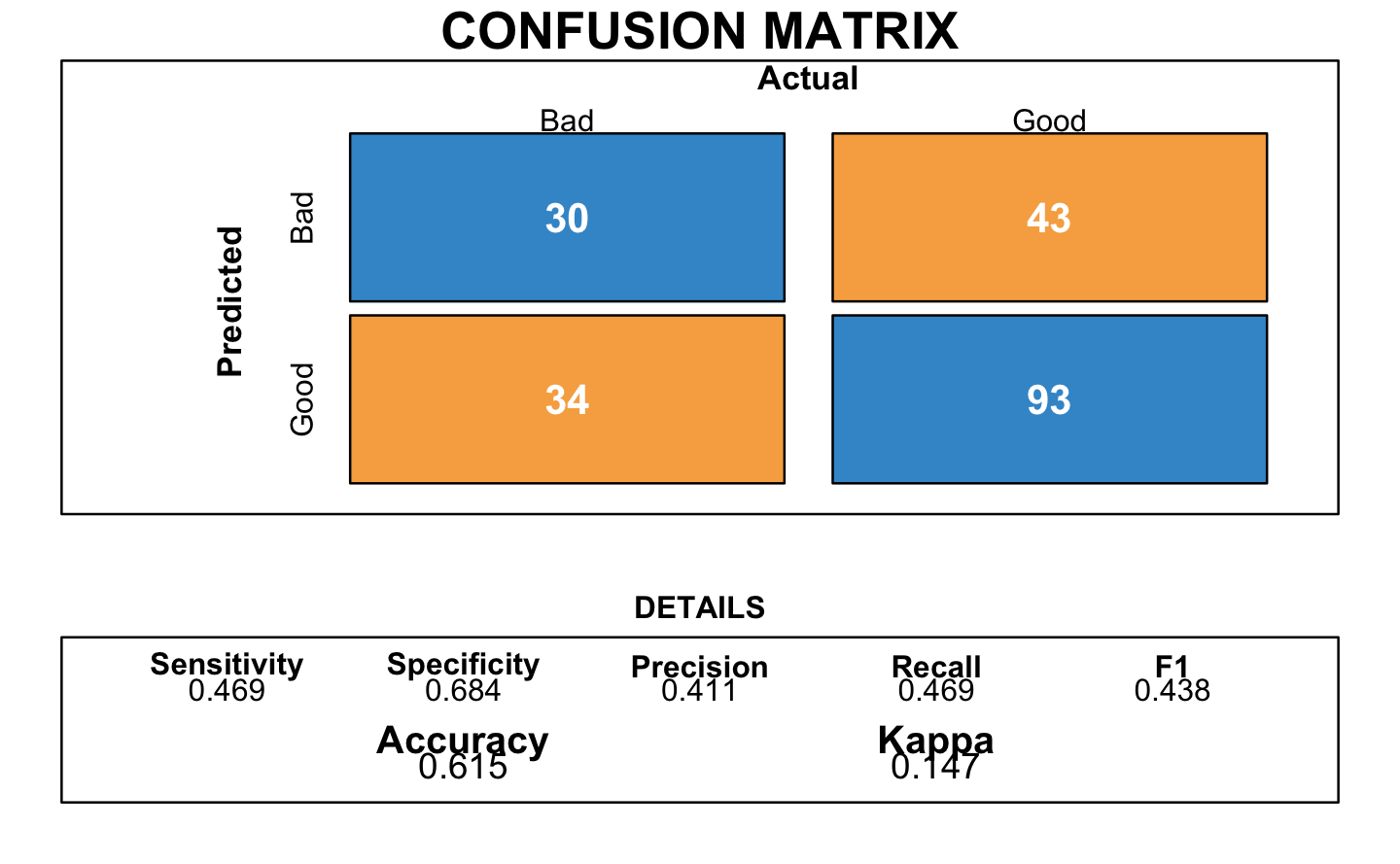
We did several confusion matrix to measure the performance. The first one was with the K-NNk method. We found an accuracy of 0.615 which corresponds to well predicted clients (good and bad). The best accuracy value is 1 so 0.615 is considered as an average value.
3.3 Naive Bayes
Then, we used a probabilistic approach with Bayes classifiers. With this method, the confusion matrix provided a better accuracy of 0.72.
# Naive Bayes

trctrl <- trainControl(method = "cv", number=10)

search_grid <- expand.grid(
  usekernel = c(TRUE, FALSE),
  laplace = 0:5,
  adjust = seq(0, 5, by = 1)
)

set.seed(346)
naive_bayes <- train(as_factor(RESPONSE) ~.,
                 data = GermanCredit.tr.subs,
                 method = "naive_bayes",
                 trControl=trctrl,
                 tuneGrid = search_grid)
3.4 Logistic Regression
A logistic regression is a regression adapted to binary classification.
We used a cross-validation method to train our model and choose the Akaïke Information Criterion (AIC) to select the variables. The AIC is used to select the model based on the number of parameters. We chose the model with the smallest AIC.
# Logistic Regression
trctrl <- trainControl(method = "cv", number=10)
set.seed(346)
glm_aic <- train(as_factor(RESPONSE) ~.,
data = GermanCredit.tr.subs,
method = "glmStepAIC",
family="binomial",
trControl=trctrl,
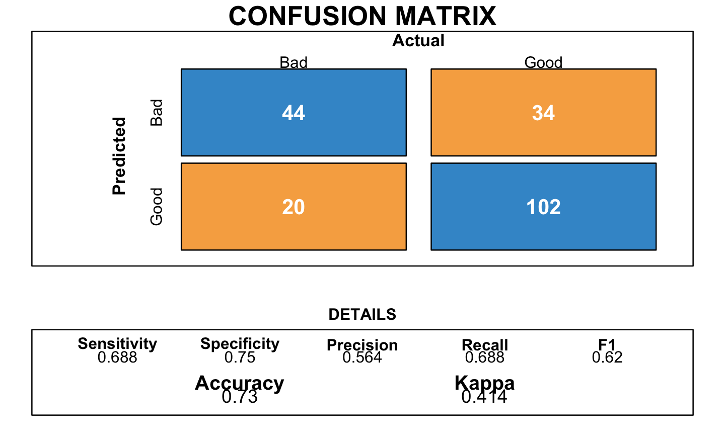
trace=0)The following plot corresponds to the resulting confusion matrix of the logistic regression:

It provided an accuracy of 0.73.
3.5 Linear Discriminant Analysis
Another model used is the Linear Discriminant Analysis.
# Linear Discriminant Analysis
trctrl <- trainControl(method = "cv", number=10)

set.seed(346)
lda.model <- train(as_factor(RESPONSE) ~.,
                 data = GermanCredit.tr.subs,
                 method = "lda",
                 trControl = trctrl)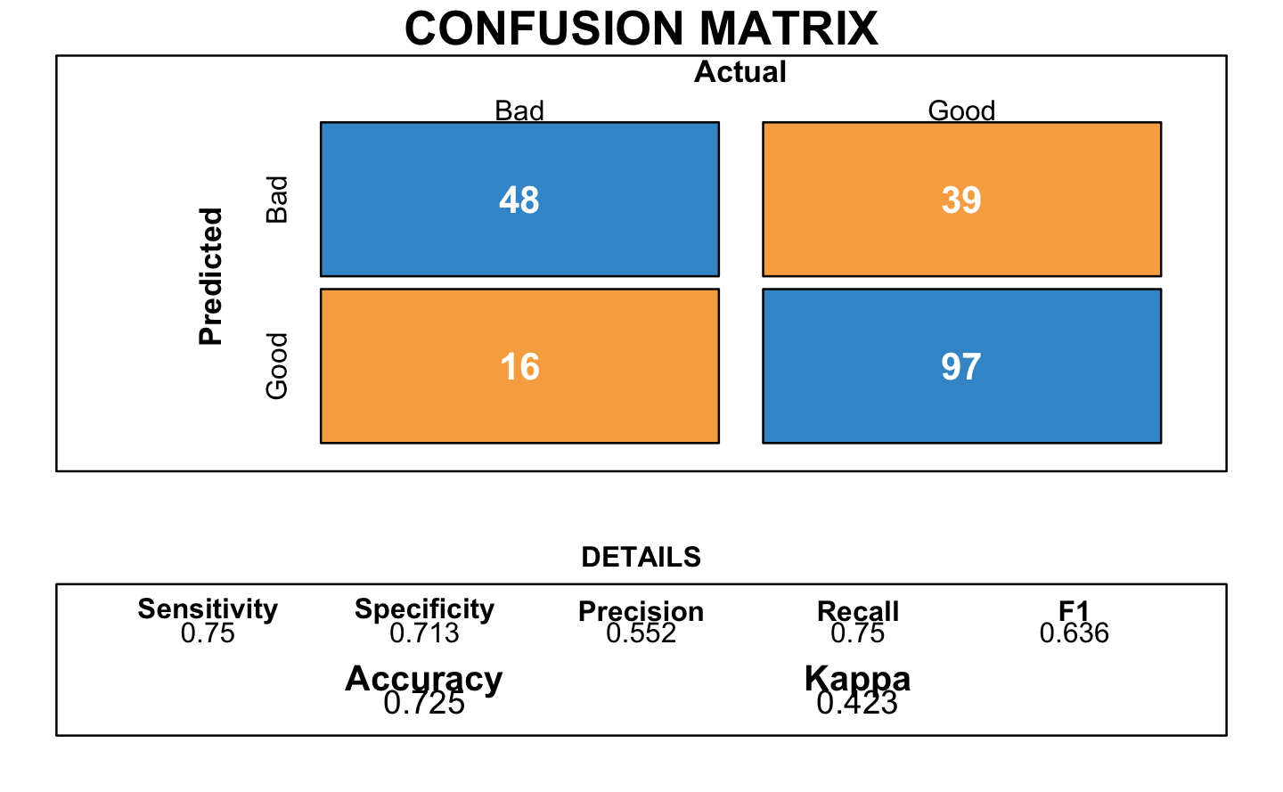
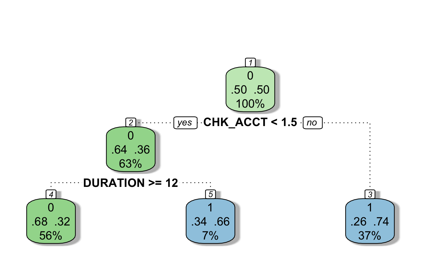
3.6 Trees
The trees represented a hierarchical set of binary rules in a shape of a tree.
# Trees

trctrl <- trainControl(method = "cv", number=10)
search_grid <- expand.grid(cp = seq(from = 0.1, to = 0, by = -0.01))

set.seed(346)
tree_model <- train(as_factor(RESPONSE) ~.,
                 data = GermanCredit.tr.subs,
                 method = "rpart",
                 trControl=trctrl,
                 tuneGrid = search_grid)
Below is a representation of the tree model:

3.7 Neural Network
Neural Network is a method based on combining several predictions of small nodes.
# Neural Network (NN)

trctrl <- trainControl(method = "cv", number=5)
search_grid <- expand.grid(size = 1:10,
                           decay = seq(0, 0.5, 0.1))

set.seed(346)
neural_network <- train(as_factor(RESPONSE) ~.,
                 data = GermanCredit.tr.subs,
                 method = "nnet",
                 trControl=trctrl,
                 tuneGrid = search_grid)
The confusion matrix with neural network presented a good accuracy of 0.705.
3.8 Random Forest
# Random Forest

trctrl <- trainControl(method = "cv", number=5)
search_grid <- expand.grid(.mtry = c(1:15))

set.seed(346)
rf <- train(as_factor(RESPONSE) ~.,
            data = GermanCredit.tr.subs,
            method = "rf",
            trControl = trctrl,
            tuneGrid = search_grid
)
Again, this models shared an accuracy of 0.73.
3.9 Summary
To evaluate our models, there are many metrics that can be used. We decided to choose first the accuracy and then have a look at the sensitivity and the specificity. In other words, we wanted to have a model with a good accuracy and the best sensitivity and specificity.
| Accuracy | Sensitivity | Specificity | |
|---|---|---|---|
| Logistic Regression | 0.73 | 0.72 | 0.74 |
| Random Forest | 0.73 | 0.69 | 0.75 |
| Linear Discriminant Analysis | 0.72 | 0.75 | 0.71 |
| Naive Bayes | 0.72 | 0.81 | 0.68 |
| Neural Network | 0.70 | 0.75 | 0.68 |
| Tree | 0.65 | 0.66 | 0.65 |
| K-nearest neighbors | 0.62 | 0.47 | 0.68 |
By looking at this summary table of the models, we can see that the Logistic Regression and the Random Forest are our top models. So, we decided to choose the following models:
- Logistic Regression
- Random Forest
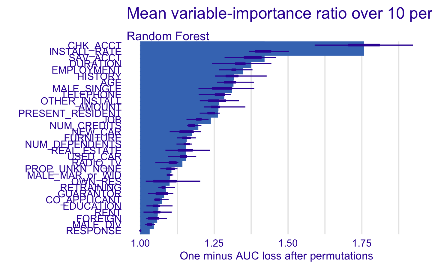
3.10 Variable Importance
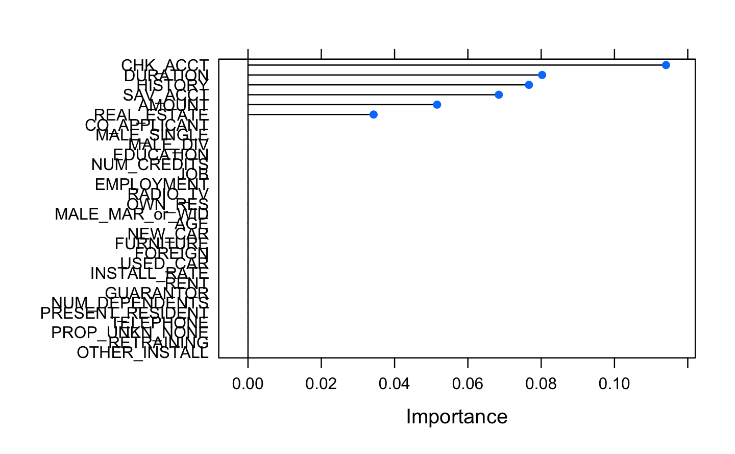
The following plot shows a selection of the most important variables of our data frame. The two main disadvantages of these methods are: The increasing over fitting risk when the number of observations is insufficient. The significant computation time when the number of variables is large.
The result below displays that we seem to have 6 relevant variables: checking account, the duration of the credit asked, the history of previous credits, the savings, the amount of money owned by the applicant and the real estate owned.
After this first global analysis, we wanted to evaluate if there is room for improvement for the models selected in Machine Learning, in other words, if we can remove some variables to make the analysis easier without loosing the performance (therefore, making the models robust)
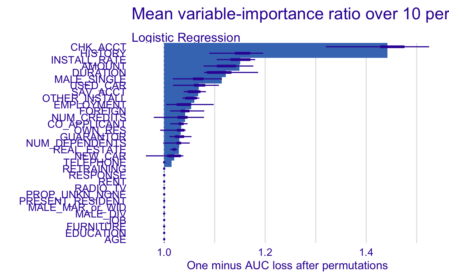
3.10.1 Logistic Regression
| Accuracy | Sensitivity | Specificity | |
|---|---|---|---|
| Original Logistic Regression | 0.73 | 0.72 | 0.74 |
| Refit Logistic Regression | 0.66 | 0.61 | 0.68 |
As we can see in the table above, we lost performance in terms of the metrics. This means that the variable importance is not that important for the logistic regression. A good point is that we need to remind ourselves that the logistic regression already does a variable importance with the AIC criterion.